In this paper some statistical properties including nature of hazard function, mean residual life function, and moments based descriptive statistical constants including coefficient of variation, skweness, kurtosis and index of dispersion of the weighted Amarendra distribution has been discussed. Two methods of estimation, namely, maximum likelihood estimation and maximum product spacing estimation have been discussed. The simulation study has been presented to know the consistency of the estimator of parameters given by the two methods of estimation. Confidence intervals of the parameters are given. The goodness of fit of the distribution has been demonstrated with two real lifetime datasets and the goodness of fit shows that weighted Amarendra distribution provides better fit over weighted Pratibha distribution, weighted Komal distribution, weighted Lindley distribution, weighted Garima distribution, weighted Sujatha distribution, weighted Akash distribution and Gamma distribution.

Keywords: amarendra distribution, hazard function, mean residual life function, moments based measures, estimation of parameters, applications

In distribution theory, it is very much useful and practical to add a shape parameter to an existing distribution using a weighted approach because the existing distribution exhibits increased flexibility and tractability tendencies with the inclusion of a shape parameter. Weighted distributions are used to model heterogeneity, clustered sampling, and extraneous variance in the dataset. Fisher¹ was the first person to introduce the concept of weighted distributions and it was Rao² who popularize the concept with several practical and real life examples with some mathematical treatment of weighted distributions. Generally, weighted versions of one parameter lifetime distributions have been derived by several researchers using the weight function $w\left(x,\alpha \right)=x^{\alpha -1}$ or $w\left(x,\alpha \right)=x^{\alpha }$ and $\alpha =1 \text{or} \alpha =0$ thus the corresponding weighted distribution will reduce to the origina distribution for. For examples, Ghitany et al³ proposed weighted Lindley distribution (WLD) from Lindley distribution of Lindley,⁴ Shanker and Shukla⁵ proposed weighted Akash distribution (WAkD) from Akash distribution of Shanker,⁶ Eyob and Shanker⁷ suggested weighted Garima distribution (WGD) from Garima distribution of Shanker,⁸ Ganaie et al.⁹ suggested weighted Aradhana distribution (WArD) from Aradhana distribution of Shanker.¹⁰ It is to be noted that the WArD derived by Ganaie et al.⁹ was having some serious drawbacks and Shanker et al.¹¹ pointed out those drawbacks of WArD and discussed several interesting properties of WArD and suggested some interesting applications. Further, Shanker and Shukla¹² suggested weighted Sujatha distribution (WSD) from Sujatha distribution of Shanker,¹³ Shanker et al.¹⁴ suggested weighted Komal distribution (WKD) from Komal distribution of Shanker,¹⁵ Shanker et al.¹⁶ suggested weighted Uma distribution (WUD) from Uma distribution of Shanker,¹⁷ Prodhani and Shanker¹⁸ suggested weighted Pratibha distribution (WPD) from Pratibha distribution of Shanker,¹⁹ respectively. While testing the goodness of fit of these weighted distributions, it has been observed that in certain datasets, these weighted distributions do not provide a suitable fit due to either distributional nature of weighted distributions or the stochastic nature of the data. Therefore, there is a need for the further weighted version of the existing distribution. Keeping this in mind, an attempt has been made to have detailed study on weighted Amarendra distribution.

Shanker¹⁹ introduced a one parameter Amarendra distribution defined by its probability density function (pdf) and cumulative density function (cdf) as

$f\left(x;\theta \right)=\frac{{\theta }^4}{{\theta }^3+{\theta }^2+2\theta +6}\left(1+x+x^2+x^3\right)x^{\alpha -1}{e}^{-\theta x};x>0,\theta >0$ $F\left(x;\theta \right)=1-\left[1+\frac{{\theta }^3{x}^3+{\theta }^2+\left(\theta +2\right)x^2+\theta \left({\theta }^3+{\theta }^2+2\theta +6\right)x}{{\theta }^3+{\theta }^2+2\theta +6}\right]e^{-\theta x};x>0,\theta >0$

Mohiuddin et al.²¹ derived weighted Amarendra distribution (WAD) using weighted technique with weight function$w\left(x\right)=x^{\alpha }$ from Amarendra distribution and discussed it statistical properties such as survival function, hazard function, Mill’s ratio, moments based measure such as mean, variance, harmonic mean, moment generating function, characteristics function , order statistics, entropy measures, Bonferroni and Lorenz curves, likelihood ratio test, maximum likelihood estimation, and represent goodness of fit on two datasets and compared WAD with Amarendra distribution and concluded that WAD provides a better fit over Amarendra distribution.

It has been observed that there are several statistical properties of WAD which has not been studied by Mohiuddin et al.²¹ including moments based measures such as coefficient of skweness, kurtosis, index of dispersion; nature of hazard function and the mean residual life function. Further, there are two serious drawbacks of the WAD proposed by Mohiuddin et al.,²¹ namely (i) The goodness of fit was compared with Amarendra distribution which is not justifiable due to the fact that a comparison of weighted distribution with unweighted distribution is completely illogical, (ii) WAD was compared with Amarendra distribution without K-S and p-value, and concluded that WAD gives better fit over Amarendra distribution, which is unreasonable and such conclusion would never be acceptable to researchers in statistics.

In this paper, a WAD is proposed using weight function$w\left(x\right)=x^{\alpha -1}$  from Amarendra distribution. Some of its important statistical properties such as hazard function, mean residual life function, moments based measures including coefficient of variation, skewness, kurtosis and index of dispersion have been derived and discussed. Parameters are estimated by the method of maximum likelihood estimation and maximum product spacing estimation. A simulation study is carried out to show the consistency of the estimator the parameters by maximum likelihood estimation and maximum product spacing estimation. Confidence interval of the parameters has been presented with profile plot of the parameters. Two real lifetime datasets have been presented to explain the applications of WAD and the goodness of fit of WAD has been compared with several weighted distributions including WPD, WKD, WLD, WGD, WSD, WAkD and gamma distribution (GD).

The weighted Amarendra distribution (WAD) can be obtained using weighted technique with weight function$w\left(x\right)=x^{\alpha -1}$  from Amarendra distribution. The pdf and cdf of WAD can be expressed as

$f\left(x;\theta ,\alpha \right)=\frac{{\theta }^{\alpha +3}\left(1+x+x^2+x^3\right)x^{\alpha -1}{e}^{-\theta x}}{\left[{\theta }^3+\alpha {\theta }^2+\alpha \left(\alpha +1\right)\theta +\alpha \left(\alpha +1\right)\left(\alpha +2\right)\right]\Gamma \left(\alpha \right)};x>0,\theta >0,\alpha >0$ $F\left(x;\theta ,\alpha \right)=1-\frac{{\theta }^3\Gamma \left(\alpha ,\theta x\right)+{\theta }^2\Gamma \left(\alpha +1,\theta x\right)+\theta \Gamma \left(\alpha +2,\theta x\right)+\Gamma \left(\alpha +3,\theta x\right)}{\left[{\theta }^3+\alpha {\theta }^2+\alpha \left(\alpha +1\right)\theta +\alpha \left(\alpha +1\right)\left(\alpha +2\right)\right]\Gamma \left(\alpha \right)};x>0,\theta >0,\alpha >0$

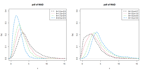
where $\theta$ is a scale parameter and $\alpha$ is shape parameter of the distribution. If we take$\alpha =\alpha +1$ , we can get the weighted Amarendra distribution proposed by Mohiuddin et al.²⁰ When $\alpha =1$ ,WAD reduces to Amarendra distribution. The behaviours of the pdf and cdf of WAD are shown in the following Figures 1 & 2 respectively. For increasing values of shape parameter $\alpha$ , kurtosis is lower and the curve tends to zero at faster rate. This shows that it positively skewed distribution and becomes symmetrical for increasing values of shape parameter $\alpha$ .

Figure 1 pdf of WAD.

Figure 2 cdf of WAD.

The r th moment about origin of WAD can be obtained as
${\mu }_r{}^{\prime }=E\left(X^r\right)={\displaystyle \underset{0}{\overset{\infty }{\int }}{x}^{r}g\left(x;\theta ,\alpha \right)dx}$
$=\frac{\left[{\theta }^3+\left(\alpha +r\right){\theta }^2+\left(\alpha +r\right)\left(\alpha +r+1\right)\theta +\left(\alpha +r\right)\left(\alpha +r+1\right)\left(\alpha +r+2\right)\right]\Gamma \left(\alpha +r\right)}{{\theta }^r\left[{\theta }^3+\alpha {\theta }^2+\alpha \left(\alpha +1\right)\theta +\alpha \left(\alpha +1\right)\left(\alpha +2\right)\right]\Gamma \left(\alpha \right)};r=1,2,\mathrm{3...}$

Putting r= 1,2,3,4 we obtain the first four moments about origin as follows ${\mu }_1{}^{\prime }=\frac{\alpha \left[{\theta }^3+\left(\alpha +1\right){\theta }^2+\left(\alpha +1\right)\left(\alpha +2\right)\theta +\left(\alpha +1\right)\left(\alpha +2\right)\left(\alpha +3\right)\right]}{\theta \left[{\theta }^3+\alpha {\theta }^2+\alpha \left(\alpha +1\right)\theta +\alpha \left(\alpha +1\right)\left(\alpha +2\right)\right]}$ ${\mu }_2{}^{\prime }=\frac{\alpha \left(\alpha +1\right)\left[{\theta }^3+\left(\alpha +2\right){\theta }^2+\left(\alpha +2\right)\left(\alpha +3\right)\theta +\left(\alpha +2\right)\left(\alpha +3\right)\left(\alpha +4\right)\right]}{{\theta }^2\left[{\theta }^3+\alpha {\theta }^2+\alpha \left(\alpha +1\right)\theta +\alpha \left(\alpha +1\right)\left(\alpha +2\right)\right]}$ ${\mu }_3{}^{\prime }=\frac{\alpha \left(\alpha +1\right)\left(\alpha +2\right)\left[{\theta }^3+\left(\alpha +3\right){\theta }^2+\left(\alpha +3\right)\left(\alpha +4\right)\theta +\left(\alpha +3\right)\left(\alpha +4\right)\left(\alpha +5\right)\right]}{{\theta }^3\left[{\theta }^3+\alpha {\theta }^2+\alpha \left(\alpha +1\right)\theta +\alpha \left(\alpha +1\right)\left(\alpha +2\right)\right]}$ ${\mu }_4{}^{\prime }=\frac{\alpha \left(\alpha +1\right)\left(\alpha +2\right)\left(\alpha +3\right)\left[{\theta }^3+\left(\alpha +4\right){\theta }^2+\left(\alpha +4\right)\left(\alpha +5\right)\theta +\left(\alpha +4\right)\left(\alpha +5\right)\left(\alpha +6\right)\right]}{{\theta }^4\left[{\theta }^3+\alpha {\theta }^2+\alpha \left(\alpha +1\right)\theta +\alpha \left(\alpha +1\right)\left(\alpha +2\right)\right]}$

Now using the relationship between raw moments and central moments we obtain the central moments of WAD as ${\mu }_2=\frac{\alpha \left(\begin{array}{l}{\alpha }^6+2{\alpha }^5\theta +3{\alpha }^4{\theta }^2+4{\alpha }^3{\theta }^3+3{\alpha }^2{\theta }^4+2\alpha {\theta }^5+{\theta }^6+9{\alpha }^5+14{\alpha }^4\theta +18{\alpha }^3{\theta }^2\\ +24{\alpha }^2{\theta }^3+9\alpha {\theta }^4+2{\theta }^5+31{\alpha }^4+34{\alpha }^3\theta +33{\alpha }^2{\theta }^2+44\alpha {\theta }^3+6{\theta }^4+51{\alpha }^3\\ +34{\alpha }^2\theta +18\alpha {\theta }^2+24{\theta }^3+40{\alpha }^2+12\alpha \theta +12\alpha \end{array}\right)}{{\theta }^2{\left({\alpha }^3+{\alpha }^2\theta +\alpha {\theta }^2+{\theta }^3+3{\alpha }^2+\alpha \theta +2\alpha \right)}^2}$ ${\mu }_3=\frac{2\alpha \left(\begin{array}{l}{\alpha }^9+3{\alpha }^8\theta +6{\alpha }^7{\theta }^2+10{\alpha }^6{\theta }^3+12{\alpha }^5{\theta }^4+12{\alpha }^4{\theta }^5+10{\alpha }^3{\theta }^6+6{\alpha }^2{\theta }^7+3\alpha {\theta }^8+{\theta }^9\\ +12{\alpha }^8+30{\alpha }^7\theta +51{\alpha }^6{\theta }^2+74{\alpha }^5{\theta }^3+81{\alpha }^4{\theta }^4+78{\alpha }^3{\theta }^5+61{\alpha }^2{\theta }^6+18\alpha {\theta }^7+3{\theta }^8\\ +60{\alpha }^7+120{\alpha }^6\theta +165{\alpha }^5{\theta }^2+198{\alpha }^4{\theta }^3+180{\alpha }^3{\theta }^4+150{\alpha }^2{\theta }^5+111\alpha {\theta }^6+12{\theta }^7\\ +162{\alpha }^6+246{\alpha }^5\theta +255{\alpha }^4{\theta }^2+238{\alpha }^3{\theta }^3+153{\alpha }^2{\theta }^4+84\alpha {\theta }^5+60{\theta }^6+255{\alpha }^5\\ +273{\alpha }^4\theta +189{\alpha }^3{\theta }^2+128{\alpha }^2{\theta }^3+42\alpha {\theta }^4+234{\alpha }^4+156{\alpha }^3\theta +54{\alpha }^2{\theta }^2+24\alpha {\theta }^3\\ +116{\alpha }^3+36{\alpha }^2\theta +24{\alpha }^2\end{array}\right)}{{\theta }^3{\left({\alpha }^3+{\alpha }^2\theta +\alpha {\theta }^2+{\theta }^3+3{\alpha }^2+\alpha \theta +2\alpha \right)}^3}$ ${\mu }_4=\frac{3\alpha \left(\begin{array}{l}{\alpha }^{13}+4{\alpha }^{12}\theta +10{\alpha }^{11}{\theta }^2+20{\alpha }^{10}{\theta }^3+31{\alpha }^9{\theta }^4+40{\alpha }^8{\theta }^5+44{\alpha }^7{\theta }^6+40{\alpha }^6{\theta }^7+31{\alpha }^5{\theta }^8\\ +20{\alpha }^4{\theta }^9+10{\alpha }^3{\theta }^{10}+4{\alpha }^2{\theta }^{11}+\alpha {\theta }^{12}+{\theta }^{13}+20{\alpha }^{12}+72{\alpha }^{11}\theta +166{\alpha }^{10}{\theta }^2+316{\alpha }^9{\theta }^3\\ +450{\alpha }^8{\theta }^4+528{\alpha }^7{\theta }^5+524{\alpha }^6{\theta }^6+408{\alpha }^5{\theta }^7+264{\alpha }^4{\theta }^8+136{\alpha }^3{\theta }^9+46{\alpha }^2{\theta }^{10}\\ +12\alpha {\theta }^{11}+2{\theta }^{12}+173{\alpha }^{11}+548{\alpha }^{10}\theta +1136{\alpha }^9{\theta }^2+2016{\alpha }^8{\theta }^3+2550{\alpha }^7{\theta }^4+2640{\alpha }^6{\theta }^5\\ +2332{\alpha }^5{\theta }^6+1560{\alpha }^4{\theta }^7+885{\alpha }^3{\theta }^8+396{\alpha }^2{\theta }^9+76\alpha {\theta }^{10}+8{\theta }^{11}+856{\alpha }^{10}+2328{\alpha }^9\theta \\ +4220{\alpha }^8{\theta }^2+6856{\alpha }^7{\theta }^3+7396{\alpha }^6{\theta }^4+6464{\alpha }^5{\theta }^5+4908{\alpha }^4{\theta }^6+2648{\alpha }^3{\theta }^7\\ +1268{\alpha }^2{\theta }^8+520\alpha {\theta }^9+40{\theta }^{10}+2691{\alpha }^9+6108{\alpha }^8\theta +9362{\alpha }^7{\theta }^2+13700{\alpha }^6{\theta }^3\\ +11955{\alpha }^5{\theta }^4+8264{\alpha }^4{\theta }^5+5136{\alpha }^3{\theta }^6+1904{\alpha }^2{\theta }^7+616\alpha {\theta }^8+240{\theta }^9+5628{\alpha }^8\\ +1029{\alpha }^7\theta +12758{\alpha }^6{\theta }^2+16572{\alpha }^5{\theta }^3+10834{\alpha }^4{\theta }^4+5296{\alpha }^3{\theta }^5+2560{\alpha }^2{\theta }^6\\ +3448\alpha {\theta }^7+7943{\alpha }^7+11180{\alpha }^6\theta +10468{\alpha }^5{\theta }^2+1912{\alpha }^4{\theta }^3+5120{\alpha }^3{\theta }^4+1344{\alpha }^2{\theta }^5\\ +480\alpha {\theta }^6+7480{\alpha }^6+7560{\alpha }^5\theta +4744{\alpha }^4{\theta }^2+4672{\alpha }^3{\theta }^3+976{\alpha }^2{\theta }^4+4504{\alpha }^5\\ +2896{\alpha }^4\theta +912{\alpha }^3{\theta }^2+768{\alpha }^2{\theta }^3+1568{\alpha }^4+480{\alpha }^3\theta +240{\alpha }^3\end{array}\right)}{{\theta }^4{\left({\alpha }^3+{\alpha }^2\theta +\alpha {\theta }^2+{\theta }^3+3{\alpha }^2+\alpha \theta +2\alpha \right)}^4}$

Thus, the coefficient of variation (C.V), coefficient of skewness$$\left(\sqrt{{\beta }_1}\right)$$, coefficient of kurtosis$\left({\beta }_2\right)$, and index of dispersion$\left(\gamma \right)$ of WAD are obtained as $CV=\frac{\sqrt{{\mu }_2}}{{\mu }_1{}^{\prime }}=\frac{\sqrt{\alpha \left(\begin{array}{l}{\alpha }^6+2{\alpha }^5\theta +3{\alpha }^4{\theta }^2+4{\alpha }^3{\theta }^3+3{\alpha }^2{\theta }^4+2\alpha {\theta }^5+{\theta }^6+9{\alpha }^5+14{\alpha }^4\theta +18{\alpha }^3{\theta }^2\\ +24{\alpha }^2{\theta }^3+9\alpha {\theta }^4+2{\theta }^5+31{\alpha }^4+34{\alpha }^3\theta +33{\alpha }^2{\theta }^2+44\alpha {\theta }^3+6{\theta }^4+51{\alpha }^3\\ +34{\alpha }^2\theta +18\alpha {\theta }^2+24{\theta }^3+40{\alpha }^2+12\alpha \theta +12\alpha \end{array}\right)}}{\alpha \left[{\theta }^3+\left(\alpha +1\right){\theta }^2+\left(\alpha +1\right)\left(\alpha +2\right)\theta +\left(\alpha +1\right)\left(\alpha +2\right)\left(\alpha +3\right)\right]}$ $$\sqrt{{\beta }_1}=\frac{{\mu }_3}{{\mu }_2{}^{\frac{3}{2}}}$$ $$=\frac{2\alpha \left(\begin{array}{l}{\alpha }^9+3{\alpha }^8\theta +6{\alpha }^7{\theta }^2+10{\alpha }^6{\theta }^3+12{\alpha }^5{\theta }^4+12{\alpha }^4{\theta }^5+10{\alpha }^3{\theta }^6+6{\alpha }^2{\theta }^7+3\alpha {\theta }^8+{\theta }^9\\ +12{\alpha }^8+30{\alpha }^7\theta +51{\alpha }^6{\theta }^2+74{\alpha }^5{\theta }^3+81{\alpha }^4{\theta }^4+78{\alpha }^3{\theta }^5+61{\alpha }^2{\theta }^6+18\alpha {\theta }^7+3{\theta }^8\\ +60{\alpha }^7+120{\alpha }^6\theta +165{\alpha }^5{\theta }^2+198{\alpha }^4{\theta }^3+180{\alpha }^3{\theta }^4+150{\alpha }^2{\theta }^5+111\alpha {\theta }^6+12{\theta }^7\\ +162{\alpha }^6+246{\alpha }^5\theta +255{\alpha }^4{\theta }^2+238{\alpha }^3{\theta }^3+153{\alpha }^2{\theta }^4+84\alpha {\theta }^5+60{\theta }^6+255{\alpha }^5\\ +273{\alpha }^4\theta +189{\alpha }^3{\theta }^2+128{\alpha }^2{\theta }^3+42\alpha {\theta }^4+234{\alpha }^4+156{\alpha }^3\theta +54{\alpha }^2{\theta }^2+24{\alpha }^3\\ +116{\alpha }^3+36{\alpha }^2\theta +24{\alpha }^2\end{array}\right)}{{\left[\alpha \left(\begin{array}{l}{\alpha }^6+2{\alpha }^5\theta +3{\alpha }^4{\theta }^2+4{\alpha }^3{\theta }^3+3{\alpha }^2{\theta }^4+2\alpha {\theta }^5+{\theta }^6+9{\alpha }^5+14{\alpha }^4\theta +18{\alpha }^3{\theta }^2\\ +24{\alpha }^2{\theta }^3+9\alpha {\theta }^4+2{\theta }^5+31{\alpha }^4+34{\alpha }^3\theta +33{\alpha }^2{\theta }^2+44\alpha {\theta }^3+6{\theta }^4+51{\alpha }^3\\ +34{\alpha }^2\theta +18\alpha {\theta }^2+24{\theta }^3+40{\alpha }^2+12\alpha \theta +12\alpha \end{array}\right)\right]}^{\frac{3}{2}}}$$ $=\frac{3\alpha \left(\begin{array}{l}{\alpha }^{13}+4{\alpha }^{12}\theta +10{\alpha }^{11}{\theta }^2+20{\alpha }^{10}{\theta }^3+31{\alpha }^9{\theta }^4+40{\alpha }^8{\theta }^5+44{\alpha }^7{\theta }^6+40{\alpha }^6{\theta }^7+31{\alpha }^5{\theta }^8\\ +20{\alpha }^4{\theta }^9+10{\alpha }^3{\theta }^{10}+4{\alpha }^2{\theta }^{11}+\alpha {\theta }^{12}+{\theta }^{13}+20{\alpha }^{12}+72{\alpha }^{11}\theta +166{\alpha }^{10}{\theta }^2+316{\alpha }^9{\theta }^3\\ +450{\alpha }^8{\theta }^4+528{\alpha }^7{\theta }^5+524{\alpha }^6{\theta }^6+408{\alpha }^5{\theta }^7+264{\alpha }^4{\theta }^8+136{\alpha }^3{\theta }^9+46{\alpha }^2{\theta }^{10}\\ +12\alpha {\theta }^{11}+2{\theta }^{12}+173{\alpha }^{11}+548{\alpha }^{10}\theta +1136{\alpha }^9{\theta }^2+2016{\alpha }^8{\theta }^3+2550{\alpha }^7{\theta }^4+2640{\alpha }^6{\theta }^5\\ +2332{\alpha }^5{\theta }^6+1560{\alpha }^4{\theta }^7+885{\alpha }^3{\theta }^8+396{\alpha }^2{\theta }^9+76\alpha {\theta }^{10}+8{\theta }^{11}+856{\alpha }^{10}+2328{\alpha }^9\theta \\ +4220{\alpha }^8{\theta }^2+6856{\alpha }^7{\theta }^3+7396{\alpha }^6{\theta }^4+6464{\alpha }^5{\theta }^5+4908{\alpha }^4{\theta }^6+2648{\alpha }^3{\theta }^7\\ +1268{\alpha }^2{\theta }^8+520\alpha {\theta }^9+40{\theta }^{10}+2691{\alpha }^9+6108{\alpha }^8\theta +9362{\alpha }^7{\theta }^2+13700{\alpha }^6{\theta }^3\\ +11955{\alpha }^5{\theta }^4+8264{\alpha }^4{\theta }^5+5136{\alpha }^3{\theta }^6+1904{\alpha }^2{\theta }^7+616\alpha {\theta }^8+240{\theta }^9+5628{\alpha }^8\\ +1029{\alpha }^7\theta +12758{\alpha }^6{\theta }^2+16572{\alpha }^5{\theta }^3+10834{\alpha }^4{\theta }^4+5296{\alpha }^3{\theta }^5+2560{\alpha }^2{\theta }^6\\ +3448\alpha {\theta }^7+7943{\alpha }^7+11180{\alpha }^6\theta +10468{\alpha }^5{\theta }^2+1912{\alpha }^4{\theta }^3+5120{\alpha }^3{\theta }^4+1344{\alpha }^2{\theta }^5\\ +480\alpha {\theta }^6+7480{\alpha }^6+7560{\alpha }^5\theta +4744{\alpha }^4{\theta }^2+4672{\alpha }^3{\theta }^3+976{\alpha }^2{\theta }^4+4504{\alpha }^5\\ +2896{\alpha }^4\theta +912{\alpha }^3{\theta }^2+768{\alpha }^2{\theta }^3+1568{\alpha }^4+480{\alpha }^3\theta +240{\alpha }^3\end{array}\right)}{{\left[\alpha \left(\begin{array}{l}{\alpha }^6+2{\alpha }^5\theta +3{\alpha }^4{\theta }^2+4{\alpha }^3{\theta }^3+3{\alpha }^2{\theta }^4+2\alpha {\theta }^5+{\theta }^6+9{\alpha }^5+14{\alpha }^4\theta +18{\alpha }^3{\theta }^2\\ +24{\alpha }^2{\theta }^3+9\alpha {\theta }^4+2{\theta }^5+31{\alpha }^4+34{\alpha }^3\theta +33{\alpha }^2{\theta }^2+44\alpha {\theta }^3+6{\theta }^4+51{\alpha }^3\\ +34{\alpha }^2\theta +18\alpha {\theta }^2+24{\theta }^3+40{\alpha }^2+12\alpha \theta +12\alpha \end{array}\right)\right]}^2}$ $\gamma =\frac{{\mu }_2}{{\mu }_1{}^{\prime }}$ $=\frac{\alpha \left(\begin{array}{l}{\alpha }^6+2{\alpha }^5\theta +3{\alpha }^4{\theta }^2+4{\alpha }^3{\theta }^3+3{\alpha }^2{\theta }^4+2\alpha {\theta }^5+{\theta }^6+9{\alpha }^5+14{\alpha }^4\theta +18{\alpha }^3{\theta }^2\\ +24{\alpha }^2{\theta }^3+9\alpha {\theta }^4+2{\theta }^5+31{\alpha }^4+34{\alpha }^3\theta +33{\alpha }^2{\theta }^2+44\alpha {\theta }^3+6{\theta }^4+51{\alpha }^3\\ +34{\alpha }^2\theta +18\alpha {\theta }^2+24{\theta }^3+40{\alpha }^2+12\alpha \theta +12\alpha \end{array}\right)}{\theta \alpha \left({\alpha }^3+{\alpha }^2\theta +\alpha {\theta }^2+{\theta }^3+3{\alpha }^2+\alpha \theta +2\alpha \right)\left[{\theta }^3+\left(\alpha +1\right){\theta }^2+\left(\alpha +1\right)\left(\alpha +2\right)\theta +\left(\alpha +1\right)\left(\alpha +2\right)\left(\alpha +3\right)\right]}$

The behaviors of coefficien of variation, coefficient of skewness, coefficient of kurtosis, index of dispersion for differnet values of the parameters of WAD are presented in the Figure 3. For fixed value of α and increasing values of θ, coefficient of variation and coefficient of kurtosis are increasing, and for fixed value of θand increasing values of αcoefficient of variation decreases and coefficient of kurtosis is first decreases after that increases like U-shape. For all values of the parameter θ and α , coefficient of skewness and index of dispersion are always decreasing.

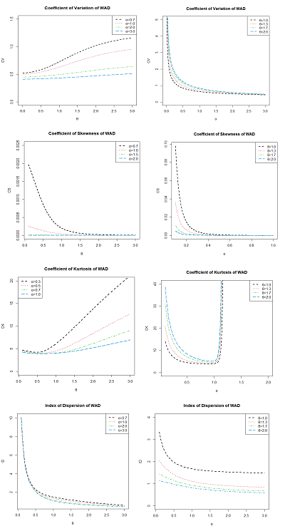
Figure 3 Graph of coefficien of variation, coefficient of skewness, coefficient of kurtosis, index of dispersion for differnet values of the parameters of WAD.

Reliability function

The survival function of the reliability function of WAD can be obtained as
$R\left(x;\theta ,\alpha \right)=1-F\left(x;\theta ,\alpha \right)$ $=\frac{{\theta }^3\Gamma \left(\alpha ,\theta x\right)+{\theta }^2\Gamma \left(\alpha +1,\theta x\right)+\theta \Gamma \left(\alpha +2,\theta x\right)+\Gamma \left(\alpha +3,\theta x\right)}{\left[{\theta }^3+\alpha {\theta }^2+\alpha \left(\alpha +1\right)\theta +\alpha \left(\alpha +1\right)\left(\alpha +2\right)\right]\Gamma \left(\alpha \right)};x>0,\theta >0,\alpha >0$

The graphical representation of reliability function is presented in Figure 4.

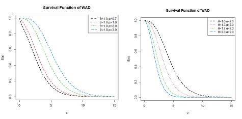
Figure 4 Survival function of WAD.

Hazard function

The hazard function of WAD can be obtained as
$h\left(x;\theta ,\alpha \right)=\frac{f\left(x;\theta ,\alpha \right)}{R\left(x;\theta ,\alpha \right)}$ $=\frac{{\theta }^{\alpha +3}\left(1+x+x^2+x^3\right)x^{\alpha -1}{e}^{-\theta x}}{{\theta }^3\Gamma \left(\alpha ,\theta x\right)+{\theta }^2\Gamma \left(\alpha +1,\theta x\right)+\theta \Gamma \left(\alpha +2,\theta x\right)+\Gamma \left(\alpha +3,\theta x\right)};x>0,\theta >0,\alpha >0$

The graphical representation of hazard function is presented in Figure 5.

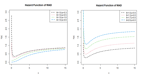
Figure 5 Hazard function of WAD.

From the Figure 5, it is clear that for any value of θ and $\alpha <1$ , it has V-shaped hazard function and for any values of θ and $\alpha \ge 1$ it has increasing hazard function.

Reverse hazard function

The reverse hazard function of WAD can be obtained as

$r\left(x;\theta ,\alpha \right)=\frac{f\left(x;\theta ,\alpha \right)}{F\left(x;\theta ,\alpha \right)}$ $=\frac{{\theta }^{\alpha +3}\left(1+x+x^2+x^3\right)x^{\alpha -1}{e}^{-\theta x}}{\left[\begin{array}{l}\left\{{\theta }^3+\alpha {\theta }^2+\alpha \left(\alpha +1\right)\theta +\alpha \left(\alpha +1\right)\left(\alpha +2\right)\right\}\Gamma \left(\alpha \right)\\ -\left\{{\theta }^3\Gamma \left(\alpha ,\theta x\right)+{\theta }^2\Gamma \left(\alpha +1,\theta x\right)+\theta \Gamma \left(\alpha +2,\theta x\right)+\Gamma \left(\alpha +3,\theta x\right)\right\}\end{array}\right]};x>0,\theta >0,\alpha >0$

Mean residual life function

The mean residual life function of WAD can be obtained as

$m\left(x;\theta ,\alpha \right)=\frac{1}{S\left(x;\theta ,\alpha \right)}{\displaystyle \underset{x}{\overset{\infty }{\int }}tf\left(t;\theta ,\alpha \right)}dt-x$

$=\frac{{\theta }^3\Gamma \left(\alpha +1,\theta x\right)+{\theta }^2\Gamma \left(\alpha +2,\theta x\right)+\theta \Gamma \left(\alpha +3,\theta x\right)+\Gamma \left(\alpha +4,\theta x\right)}{{\theta }^3\Gamma \left(\alpha ,\theta x\right)+{\theta }^2\Gamma \left(\alpha +1,\theta x\right)+\theta \Gamma \left(\alpha +2,\theta x\right)+\Gamma \left(\alpha +3,\theta x\right)}-x;x>0,\theta >0,\alpha >0$

The graphical representation of mean residual life function is presented in Figure 6.

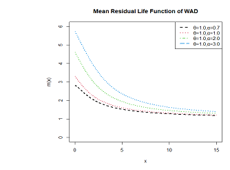
Figure 6 Mean residual life function of WAD.

Maximum Likelihood Estimation

Let $\left(x_1,x_2,\mathrm{...},x_n\right)$ be a random sample from WAD. The log-likelihood function of WAD can be expressed as

$\begin{array}{l}\log L=n\left[\left(\alpha +3\right)\log \eta -\log \left({\theta }^3+\alpha {\theta }^2+\alpha \left(\alpha +1\right)\theta +\alpha \left(\alpha +1\right)\left(\alpha +2\right)\right)\right]\\ -n\log \left(\Gamma \left(\alpha \right)\right)+{\displaystyle \sum _{i=1}^n\log \left(1+x_i+\text{}\text{}{x}_i{}^2+x_i{}^3\right)}+\left(\alpha -1\right){\displaystyle \sum _{i=1}^n\log \left(x_i\right)}-\theta \overline{x}\end{array}$

This gives
$\frac{\partial \log L}{\partial \theta }=\frac{n\left(\alpha +3\right)}{\theta }-\frac{n\left\{3{\theta }^2+2\alpha \theta +\alpha \left(\alpha +1\right)\right\}}{{\theta }^3+\alpha {\theta }^2+\alpha \left(\alpha +1\right)\theta +\alpha \left(\alpha +1\right)\left(\alpha +2\right)}-n\overline{x}=0$ $\frac{\partial \log L}{\partial \alpha }=n\log \theta -\frac{n\left\{{\theta }^2+\left(2\alpha +1\right)\theta +\left(3{\alpha }^2+6\alpha +2\right)\right\}}{{\theta }^3+\alpha {\theta }^2+\alpha \left(\alpha +1\right)\theta +\alpha \left(\alpha +1\right)\left(\alpha +2\right)}+n\psi \left(\alpha \right)+{\displaystyle \sum _{i=1}^n\log x_i}=0$

The log-likelihood equations presented here are not readily solvable because it is not in closed form, necessitating the use of maximization techniques using R software. Iterative solutions are employed to optimize the likelihood function until sufficiently close parameter values are achieved. These equations can be solved using Fisher’s scoring method. For Fisher's scoring method, the following approach is undertaken
$\frac{{\partial }^2\log L}{\partial {\theta }^2}=-\frac{n\left(\alpha +3\right)}{{\theta }^2}-\frac{n\left[\left\{{\theta }^3+\alpha {\theta }^2+\alpha \left(\alpha +1\right)\theta +\alpha \left(\alpha +1\right)\left(\alpha +2\right)\right\}\left(6\theta +2\alpha \right)-{\left\{3{\theta }^2+2\alpha \theta +\alpha \left(\alpha +1\right)\right\}}^2\right]}{{\left[{\theta }^3+\alpha {\theta }^2+\alpha \left(\alpha +1\right)\theta +\alpha \left(\alpha +1\right)\left(\alpha +2\right)\right]}^2}$ $\frac{{\partial }^2\log L}{\partial \theta \partial \alpha }=-\frac{n}{\theta }-\frac{n\left[\begin{array}{l}\left\{{\theta }^3+\alpha {\theta }^2+\alpha \left(\alpha +1\right)\theta +\alpha \left(\alpha +1\right)\left(\alpha +2\right)\right\}\left(2\theta +2\alpha +1\right)\\ -n\left\{3{\theta }^2+2\alpha \theta +\alpha \left(\alpha +1\right)\right\}\left\{{\theta }^2+\left(2\alpha +1\right)+\left(3{\alpha }^2+6\alpha +2\right)\right\}\end{array}\right]}{{\left[{\theta }^3+\alpha {\theta }^2+\alpha \left(\alpha +1\right)\theta +\alpha \left(\alpha +1\right)\left(\alpha +2\right)\right]}^2}=\frac{{\partial }^2\log L}{\partial \alpha \partial \theta }$ $\frac{{\partial }^2\log L}{\partial {\alpha }^2}=-\frac{n\left[\left\{{\theta }^3+\alpha {\theta }^2+\alpha \left(\alpha +1\right)\theta +\alpha \left(\alpha +1\right)\left(\alpha +2\right)\right\}\left(2\theta +6\alpha +6\right)-{\left\{{\theta }^2+\left(2\alpha +1\right)+\left(3{\alpha }^2+6\alpha +2\right)\right\}}^2\right]}{{\left[{\theta }^3+\alpha {\theta }^2+\alpha \left(\alpha +1\right)\theta +\alpha \left(\alpha +1\right)\left(\alpha +2\right)\right]}^2}+n{\psi }^{\prime }\left(\alpha \right)$

For finding the MLEs $\left(\widehat{\theta },\widehat{\alpha }\right)$ of parameters $$\left(\theta ,\alpha \right)$$ of WAD, following equations can be solved
${\left(\begin{array}{cc}\frac{{\partial }^2\log L}{\partial {\theta }^2}& \frac{{\partial }^2\log L}{\partial \theta \partial \alpha }\\ \frac{{\partial }^2\log L}{\partial \theta \partial \alpha }& \frac{{\partial }^2\log L}{\partial {\alpha }^2}\end{array}\right)}_{\begin{array}{l}\widehat{\theta }={\theta }_0\\ \widehat{\alpha }={\alpha }_0\end{array}}\left(\begin{array}{l}\widehat{\theta }-{\theta }_0\\ \widehat{\alpha }-{\alpha }_0\end{array}\right)=\left(\begin{array}{l}\frac{\partial \log L}{\partial \theta }\\ \frac{\partial \log L}{\partial \alpha }\end{array}\right)$

where${\theta }_0$ and are the initial values of θ and α;. These equations are solved iteratively till close estimates of parameters are obtained.

Maximum product spacing estimation

The maximum product spacing estimates (MPSE) $\left(\widehat{\theta },\widehat{\alpha }\right)$ of parameters $\left(\theta ,\alpha \right)$ can be obtained numerically by maximizing the following function with respect to θ and α.
$MPSE=\frac{1}{n+1}{\displaystyle \sum _{i=1}^{n+1}\log \left[F\left(x_i,\theta ,\alpha \right)-F\left(x_{i-1},\theta ,\alpha \right)\right]}$

To assess the consistency of maximum likelihood estimators (MLE) and maximum product spacing estimators (MPSE) for WAD, a simulation study has been conducted. The investigation involved examining mean estimates, biases (B), mean square errors (MSEs), and variances of the MLE and MPSE for WAD, utilizing the specified formulas.

$$\begin{array}{l}\text{Mean}=\frac{1}{n}{\displaystyle \sum _{i=1}^n{\widehat{H}}_i}, \text{} B=\frac{1}{n}{\displaystyle \sum _{i=1}^n\left({\widehat{H}}_i-H\right)}, \text{MSE}=\frac{1}{n}{\displaystyle \sum _{i=1}^n{\left({\widehat{H}}_i-H\right)}^2},\\ \text{Variance}=MSE-B^2\end{array}$$

where $H=\left(\theta ,\alpha \right)$ and ${\widehat{H}}_i=\left({\widehat{\theta }}_i,{\widehat{\alpha }}_i\right)$ .

The acceptance-rejection method of simulation study has been employed to generate data. This method is commonly used in simulation studies to produce random samples from a target distribution. The method for generating random samples from the WAD involves the following steps:

1. Generate Y from exponential $\left(\theta \right)$ distribution
2. Generates U from Uniform (0,1) distribution
3. If $U\le \frac{f(y)}{Mg(y)}$ , then set $X=Y$ (“accept the sample”); otherwise (“reject the sample”) and if reject then repeat the process: step (a-c) until getting the required samples. Where $M$ is a constant.
4. Each sample size is replicated 10000 times

The biases and MSEs of the MLE and MPSE of the parameters decreases for increasing sample size as evident in Table 1. This supports the first-order asymptotic theory of MLE. From the Table 1, it observed that in case of the parameter θ , MLE provides the better estimate as compared to MPSE and in case of the parameter α, MPSE provides the better estimate as compared to MLE.

Variance-Covariance matrix for the parameters $\theta =1.5, \alpha =1$ and $\theta =1.7, \alpha =2.3$ are given by

$\begin{array}{l} \theta \alpha \\ \begin{array}{c}\theta \\ \alpha \end{array}\left(\begin{array}{cc}\text{0}\text{.00013}& \text{0}\text{.00006}\\ \text{0}\text{.00006}& 0.00020\end{array}\right)\end{array}$ and $\begin{array}{l} \theta \alpha \\ \begin{array}{c}\theta \\ \alpha \end{array}\left(\begin{array}{cc}\text{0}\text{.00020}& \text{0}\text{.00003}\\ \text{0}\text{.00003}& 0.00066\end{array}\right)\end{array}$

To test the goodness of fit of WAD , we have considered following two real lifetime datasets.

Dataset 1: The following symmetric data, discussed by Murthy et al,²¹ relating to the failure times of windshields. The values are as follows.

0.04, 0.3, 0.31, 0.557, 0.943, 1.07, 1.124, 1.248, 1.281, 1.281, 1.303, 1.432, 1.48, 1.51, 1.51,1.568, 1.615, 1.619, 1.652, 1.652, 1.757, 1.795, 1.866, 1.876, 1.899, 1.911, 1.912, 1.9141,0.981, 2.010, 2.038, 2.085, 2.089, 2.097, 2.135, 2.154, 2.190, 2.194, 2.223, 2.224, 2.23, 2.3,2.324, 2.349, 2.385, 2.481, 2.610, 2.625, 2.632, 2.646, 2.661, 2.688, 2.823, 2.89, 2.9, 2.934,2.962, 2.964, 3, 3.1, 3.114, 3.117, 3.166, 3.344, 3.376, 3.385, 3.443, 3.467, 3.478, 3.578,3.595, 3.699, 3.779, 3.924, 4.035, 4.121, 4.167, 4.240, 4.255, 4.278, 4.305, 4.376, 4.449,4.485, 4.570, 4.602, 4.663, 4.694.

The total time to test (TTT) plots and the histogram of the original dataset 1 and the corresponding simulated dataset are shown in the Figure 7.

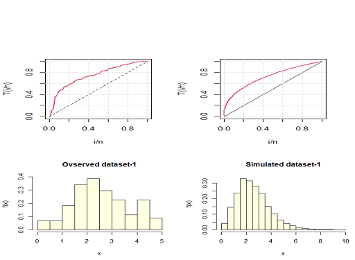
Figure 7 TTT-plot and histogram of the observed and theoretical values of the dataset-1.

Dataset-2: The following bi-modal, a set of complete data discussed by Murthy et al²² reports the lifetimes of 20 electronic components. The observations are:

0.03, 0.12, 0.22, 0.35, 0.73, 0.79, 1.25, 1.41, 1.52, 1.79, 1.80, 1.94, 2.38, 2.40, 2.87, 2.99,3.14, 3.17, 4.72, 5.09.

The total time to test (TTT) plots and the histogram of the original dataset 2 and the corresponding simulated dataset are shown in the Figure 8.

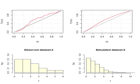
Figure 8 TTT-plot and histogram of the observed and theoretical values of the dataset-2.

In order to compare lifetime distributions, values of^{$-2\log L$} , Akaike Information Criterion (AIC), Bayesian Information Criterion (BIC), Consistent Akaike Information Criterion (CAIC), Hannan-Quinn Information Criterion (HQIC), Kolmogorov-Smirnov Statistics (K-S) and the corresponding probability value (p-value) for the above data set has been computed. The formulae for computing AIC, BIC, CAIC, HQIC and K-S are as follows:

$AIC=-2\log L+2p$ ,$BIC=-2\log L+p\log \left(n\right)$ ,$CAIC=-2\log L+\frac{2pn}{n-p-1}$

$HQIC=-2\log L+2p\log \left[\log \left(n\right)\right]$ ,$K\text{-}S=\underset{x}{Sup}|F_m\left(x\right)-F_o\left(x\right)|$

where,p= number of parameters, n= sample size, $F_m\left(x\right)=$ empirical cdf of considered distribution and $F_o\left(x\right)=$ cdf of considered distribution.

The ML estimates and the MPS estimates of the parameters along with their standard errors (in parenthesis) of the considered distributions for datasets 1 and 2 are given in Tables 2 & 3 respectively. The goodness of fit measures for the datasets 1 and 2 for the considered distributions are presented in Tables 4 & 5 respectively. It is clear from tables 4 and 5 that WAD has the least, AIC, BIC, CAIC, HQIC and K-S values as compared to the WPD, WKD, WLD, WGD, WSD, WAkD and GD, therefore WAD provides the best fit as compared to these considered distributions for the two datasets. The fitted plot of the considered distributions, Q-Q plot, P-P plot and ECDF plot of the dataset-1 and 2 are shown in the Figure 9, which also support the hypothesis that WAD provides best fit among the considered distributions. The confidence Interval of the parameters of WAD for the dataset-1 & 2 are given in Table 6. The profile plots of WAD for the datasets 1 and 2 are given in Figure 10.

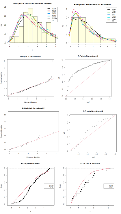
Figure 9 Fitted plot of the considered distributions, Q-Q plot, P-P plot and ECDF plot of the dataset-1 and 2 respectively.

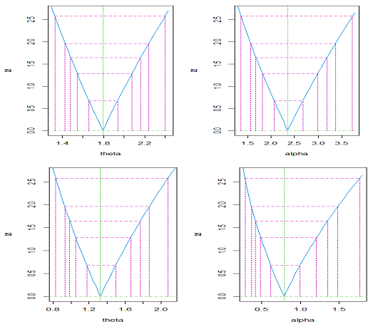
Figure 10 Profile plot of WAD for the dataset-1 and 2.

In this paper, a weighted Amarendra distribution (WAD) has been suggested which contains Amarendra distribution. Its statistical properties including moments based measures such as moments about origin, moments about mean, coefficient of variation, skewness, kurtosis, index of dispersion, reliability function, hazard function, reverse hazard function, mean residual life function have been discussed with graphical representation. Parameters are estimated by the method of maximum likelihood estimation and maximum product spacing estimation. A simulation study is carried out to show the consistency of the estimaor of the parameters by maximum likelihood estimation and maximum product spacing estimation. Confidence interval of the parameters has been presented with profile plot of the parameters. Finally, in application portion, goodness of fit demonstrated on two real lifetime datasets from engineering field and fitted plot of the considered distributions, P-P plot, Q-Q plot, and ECDF plot of dataset-1 and 2 are presented. Its shows that WAD provides a better fit as compared with WPD, WKD, WLD, WGD, WSD, WAkD and GD.

Authors are grateful to the editor in chief and the anonymous reviewer for some minor comments which improved both the quality and the presentation.

The authors declare that they have no conflicts of interest.

None.

1. Fisher RA. The effects of methods of ascertainment upon the estimation of frequencies. The Annals of Eugenics. 1934;6:13–25.
2. Rao CR. On discrete distributions arising out of methods of ascertainment. Sankhyā: The Indian Journal of Statistics, Series A. 1965;(27):311–324.
3. Ghitany ME, Alqallaf F, Al-Mutairi DK, et al. A two-parameter weighted Lindley distribution and its applications to survival data. Mathematics and Computers in Simulation. 2011;81(6):1190–1201.
4. Lindley DV. Fiducial distributions and Bayes’ theorem. Journal of the Royal Statistical Society, Series B. 1958;20(1):102–107.
5. Shanker R, Shukla KK. Weighted Akash distribution and its application to model lifetime data. International Journal of Statistics. 2016;39(2):1138–1147.
6. Shanker R. Akash distribution and its application. International Journal of Probability and Statistics. 2015;4(3):65–75.
7. Eyob T, Shanker R. A two-parameter weighted Garima distribution with properties and application. Biom Biostat Int J. 2018;7(3):234–242.
8. Shanker R. Garima distribution and Its Application to model behavioural science data. Biom Biostat Int J. 2016(a);4(7):275–281.
9. Ganaie RA, Rajagopalan V, Rather AA. Weighted Aradhana distribution: properties and applications. Journal of Information and Computational Science. 2019;9(8):392–406.
10. Shanker R. Aradhana distribution and its applications. International Journal of Statistics and Applications. 2016(b);6(1):23–34.
11. Shanker R. Uma distribution with properties and applications. Biom Biostat Int J. 2022;11(5):165–169.
12. Shanker R, Shukla KK. A two -parameter weighted Sujatha distribution and its application to model life time data. International Journal of Mathematics and Statistics. 2018;57(3):106–121.
13. Shanker R. Sujatha distribution and its application. Statistics in Transition New Series. 2016(c);17(3):391–410.
14. Shanker R, Ray M, Prodhani HR. Weighted Komal distribution with properties and applications. International Journal of Statistics and Reliability Engineering. 2023;10(3):541–551.
15. Shanker R. Komal distribution with properties and application in survival analysis. Biom Biostat Int J. 2023;12(2):40–44.
16. Shanker R, Shukla KK, Shanker R. A note on weighted Aradhana distribution with an application. Biom Biostat Int J. 2022;11(1):22–26.
17. Prodhani HR, Shanker R. Weighted Pratibha distribution with properties and application in flood dataset. Biom Biostat Int J. 2024;13(2):52–57.
18. Shanker R. Pratibha distribution with statistical properties and application. Biom Biostat Int J. 2023;12(5):136–142.  
19. Shanker R. Amarendra distribution and its applications. American Journal of Mathematics and Statistics. 2016d;6:44–56.
20. Mohiuddin M, Dar SA, Khan AA, et al. Weighted Amarendra distribution: properties and application to model real-life data. J Stat Appl Pro. 2022;11(3):1075–1093.
21. Murthy DNP, Xie M, Jiang R. Weibull models. John Wiley & Sons Inc, Hoboken. 2004.