A two–parameter weighted Garima distribution with properties and application

doi:10.15406/bbij.2018.07.00214

eISSN: 2378-315X

Biometrics & Biostatistics International Journal

Research Article Volume 7 Issue 3

A two–parameter weighted Garima distribution with properties and application

Tesfalem Eyob, Rama Shanker

Verify Captcha

Regret for the inconvenience: we are taking measures to prevent fraudulent form submissions by extractors and page crawlers. Please type the correct Captcha word to see email ID.

Department of Statistics, Eritrea Institute of Technology, Eritrea

Correspondence: Rama Shanker, Department of Statistics, Eritrea Institute of Technology, Eritrea

Received: May 03, 2018 | Published: June 13, 2018

Citation: Eyob T, Shanker R. A two–parameter weighted Garima distribution with properties and application. Biom Biostat Int J. 2018;7(3):234-242. DOI: 10.15406/bbij.2018.07.00214

Download PDF

Abstract

In this paper a two–parameter weighted Garima distribution which includes one–parameter Garima distribution has been proposed for modeling real lifetime data. Statistical properties of the distribution including shapes of probability density function, moments and moment related measures, hazard rate function, mean residual life function and stochastic orderings have been discussed. The estimation of its parameters has been discussed using the method of maximum likelihood. Application of the proposed distribution has been discussed.

Keywords: garima distribution, moments, hazard rate function, mean residual life function, stochastic ordering, maximum likelihood estimation, goodness of fit

Introduction

Fisher¹ firstly introduced the idea of weighted distributions to model ascertainment biases which were later reformulated by Rao² in a unifying theory for problems where the observations fall in non–experimental, non–replicated and non–random. When a researcher collects observations in the nature according to certain stochastic model, the distribution of the collected observations will not have the original distribution unless every observation has been given an equal chance of being included. Suppose the original observation $x_{0}$ $x_{0}$ comes from a population having a probability density function (pdf.), $f_{o} (x, θ_{1})$ $f_{o} (x, θ_{1})$ , where $θ_{1}$ $θ_{1}$ may be a parameter vector; and observation $x$ $x$ is collected according to a probability re–weighted with a weight function $w (x, θ_{2}) > 0$ $w (x, θ_{2}) > 0$ , $θ_{2}$ $θ_{2}$ being a new parameter vector, then $x$ $x$ comes from a population having pdf

$f (x; θ_{1}, θ_{2}) = k . w (x; θ_{2}) f_{o} (x; θ_{2})$ $f (x; θ_{1}, θ_{2}) = k . w (x; θ_{2}) f_{o} (x; θ_{2})$ (1.1)

where $k$ $k$ is a normalizing constant. Recall that such types of distributions are known as weighted distributions. A weighted distribution having weight function $w (x, θ_{2}) = x$ $w (x, θ_{2}) = x$ is called length–biased distribution. Extensive discussions on some general probability models leading to weighted probability distributions and their applications and the occurrence of $⌢ θ$ $\overset{⌢}{θ}$ in the problems in sampling have been discussed by Patil & Rao.^3,4

Shanker⁵ proposed a lifetime distribution named Garima distribution for modeling behavioral Science data and defined by its pdf and cumulative distribution function (cdf)

$f_{1} (x; θ) = \frac{θ}{θ + 2} (1 + θ + θ x) e^{- θ x}; x > 0, θ > 0$ $f_{1} (x; θ) = \frac{θ}{θ + 2} (1 + θ + θ x) e^{- θ x}; x > 0, θ > 0$ (1.2)

$F_{1} (x, θ) = 1 - [1 + \frac{θ x}{θ + 2}] e^{- θ x}; x > 0, θ > 0$ $F_{1} (x, θ) = 1 - [1 + \frac{θ x}{θ + 2}] e^{- θ x}; x > 0, θ > 0$ (1.3)

The first four raw moments (moments about origin) of Garima distribution obtained by Shanker⁵ are

$μ_{1}^{'} = \frac{θ + 3}{θ (θ + 2)}, μ_{2}^{'} = \frac{2 (θ + 4)}{θ^{2} (θ + 2)}, μ_{3}^{'} = \frac{6 (θ + 5)}{θ^{3} (θ + 2)}, μ_{4}^{'} = \frac{24 (θ + 6)}{θ^{4} (θ + 2)}$ $μ_{1}^{'} = \frac{θ + 3}{θ (θ + 2)}, μ_{2}^{'} = \frac{2 (θ + 4)}{θ^{2} (θ + 2)}, μ_{3}^{'} = \frac{6 (θ + 5)}{θ^{3} (θ + 2)}, μ_{4}^{'} = \frac{24 (θ + 6)}{θ^{4} (θ + 2)}$

The central moments (moments about the mean) of Garima distribution obtained by Shanker⁵ are given by

$\begin{array}{l} μ_{2} = \frac{θ^{2} + 6 θ + 7}{θ^{2} {(θ + 2)}^{2}} \\ μ_{3} = \frac{2 (θ^{3} + 9 θ^{2} + 21 θ + 15)}{θ^{3} {(θ + 2)}^{3}} \\ μ_{4} = \frac{3 (3 θ^{4} + 36 θ^{3} + 134 θ^{2} + 204 θ + 111)}{θ^{4} {(θ + 2)}^{4}} \end{array}$

Statistical properties including shapes for different values of parameter, hazard rate function, mean residual life function, stochastic ordering, mean deviations, order statistic, Bonferroni and Lorenz curves, Renyi entropy measures and stress–strength reliability of Garima distribution have been discussed in Shanker.⁵ Estimation of parameter using both the method of moment and the method of maximum likelihood along with application of Garima distribution has been explained in Shanker.⁵ The suitability, superiority and application of Garima distribution for modeling behavioral science data over exponential and Lindley distribution, introduced by Lindley,⁶ have also been discussed by Shanker.⁵ Ghitany et al.,⁷ have detailed study on statistical properties, estimation of parameter and application of Lindley distribution to model waiting time in a bank and established that Lindley distribution gives much closer fit than exponential distribution. Further, Ghitany et al.,⁸ introduced a two–parameter weighted Lindley distribution (WLD) defined by its pdf and cdf

$f_{2} (x; θ, β) = \frac{θ^{β + 1}}{(θ + β) Γ (β)} x^{β - 1} (1 + x) e^{- θ x}; x > 0, θ > 0, β > 0$ (1.4)

$F_{2} (x; θ, β) = 1 - \frac{(θ + β) Γ (β, θ x) + {(θ x)}^{β} e^{- θ x}}{(θ + β) Γ (β)}; x > 0, θ > 0, β > 0$ (1.5)

where $Γ (β, θ x)$ is the upper incomplete gamma function defined as

$Γ (β, z) = \int_{z}^{\infty} e^{- y} y^{β - 1} d y; y \geq 0, β > 0$ (1.6)

It can be easily shown that Lindley distribution is a particular case of WLD at $β = 1$ . Shanker et al.,⁹ proposed an extension of WLD named a three–parameter weighted Lindley distribution which includes Lindley distribution and WLD as particular cases.

Shanker¹⁰ has obtained discrete Poisson–Garima distribution (PGD), discussed its statistical properties, estimation of parameter and applications for count data from biological sciences. Shanker & Shukla^11,12 have also proposed size–biased Poisson–Garima distribution (SBPGD) and Zero–truncated Poisson–Garima distribution (ZTPGD), along with estimation of their parameter and applications for data which structurally excludes zero counts.

The organizations of the rest of the paper are as follows: Section 2 deals with two–parameter weighted Garima distribution (WGD) which includes one–parameter Garima distribution proposed by Shanker⁵ along with the shapes of the pdf and the cdf of WGD. Section 3 deals with statistical constants and associated measures of WGD including coefficient of variation, skewness, kurtosis, index of dispersion. Section 4 deals with the reliability properties of WGD including hazard rate function, mean residual life function and stochastic ordering. Section 5 deals with the maximum likelihood method for the estimation of parameters of the distribution. Section 6 deals with the goodness of fit of the proposed distribution with a real lifetime data over other one parameter and two–parameter lifetime distributions. Finally, the conclusions of the paper have been presented in section 7.

Weighted Garima distribution

The pdf of the weighted Garima distribution (WGD) can be expressed as

$f_{3} (x; θ, β) = K x^{β - 1} f_{o} (x; θ); x > 0, θ > 0, β > 0$ (2.1)

where, K is the normalizing constant and $f_{o} (x; θ)$ is the pdf of Garima distribution given in (1.2). Thus the pdf of WGD can be obtained as

$f_{3} (x; θ, β) = \frac{θ^{β}}{(θ + β + 1)} \frac{x^{β - 1}}{Γ (β)} (1 + θ + θ x) e^{- θ x}; x > 0, θ > 0, β > 0$ (2.2)

where

$Γ (β) = \int_{0}^{\infty} e^{- y} y^{β - 1} d y; y > 0, β > 0$ is the complete gamma function.

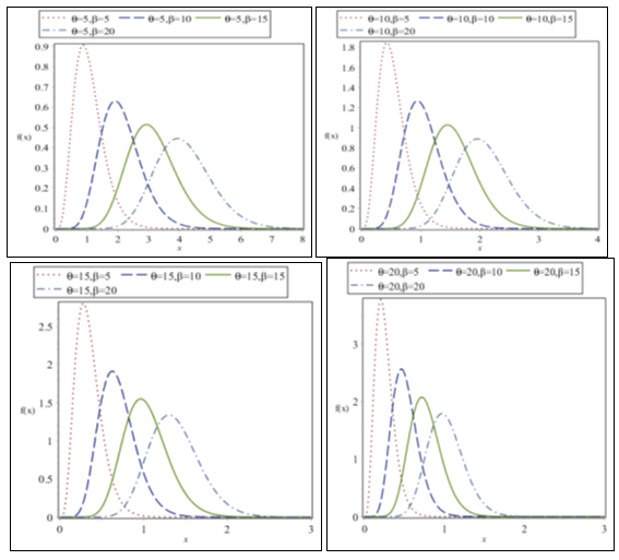
We say that $X$ follows WGD with parameters $θ$ and $β$ if its pdf is given by (2.2) and we denote it by $X ~ WGD (θ, β)$ . It can be easily verified that Garima distribution and size–biased Garima distribution (SBGD) are particular cases of WGD at $β = 1$ and $β = 2$ , respectively. The behavior of the pdf of WGD for different combinations of parameters $θ$ and $β$ are shown in Figure 1.

Figure 1 Behavior of the pdf of WGD for different combinations of the parameters

$θ$ and

$β$ .

The cdf of the WGD can be expressed as

$F_{3} (x; θ, β) = 1 - \frac{{(θ x)}^{β} e^{- θ x} + (θ + β + 1) Γ (β, θ x)}{(θ + β + 1) Γ (β)}; x > 0, θ > 0, β > 0$ (2.3)

where $Γ (β, θ x)$ is the upper incomplete gamma function defined in (1.6). Behavior of the cdf of the WGD for different combinations of the parameters $θ$ and $β$ are shown in Figure 2.

Figure 2 Behavior of the cdf of WGD for different combinations of the parameters

$θ$ and

$β .$

Statistical constants and related measures

The rth raw moments (moment about origin), $μ_{r}^{'}$ ,of WGD (2.2) can be derived as

$μ_{r}^{'} = E (X^{r}) = \int_{0}^{\infty} x^{r} f_{2} (x; θ, β) d x = \int_{0}^{\infty} x^{r} \frac{x^{β - 1}}{(θ + β + 1)} \frac{θ^{β}}{Γ (β)} (1 + θ + θ x) e^{- θ x} d x$

$= \frac{(θ + β + r + 1) Γ (β + r)}{θ^{r} (θ + β + 1) Γ (β)}; r = 1, 2, 3, . . .$ (3.1)

Thus the first four raw moments of WGD are obtained as

$μ_{1}^{'} = \frac{β (θ + β + 2)}{θ (θ + β + 1)}$

$μ_{2}^{'} = \frac{β (β + 1) (θ + β + 3)}{θ^{2} (θ + β + 1)}$

$μ_{3}^{'} = \frac{β (β + 1) (β + 2) (θ + β + 4)}{θ^{3} (θ + β + 1)}$

$μ_{4}^{'} = \frac{β (β + 1) (β + 2) (β + 3) (θ + β + 5)}{θ^{4} (θ + β + 1)}$

Using relationship $μ_{r} = E {(X - μ_{1}^{'})}^{r} = \sum_{k = 0}^{r} (\begin{array}{l} r \\ k \end{array}) μ_{k}^{'} {(- μ_{1}^{'})}^{r - k}$ between central moments and raw moments, the central moments of WGD are

$μ_{2} = \frac{β {θ^{2} + (2 β + 4) θ + (β^{2} + 3 β + 3)}}{θ^{2} {(θ + β + 1)}^{2}}$

$μ_{3} = \frac{2 β {θ^{3} + (3 β + 6) θ^{2} + (3 β^{2} + 9 β + 9) θ + (β^{3} + 4 β^{2} + 6 β + 4)}}{θ^{3} {(θ + β + 1)}^{3}}$

$μ_{4} = \frac{3 β {\begin{cases} (β + 2) θ^{4} + (4 β^{2} + 16 β + 16) θ^{3} + (6 β^{3} + 34 β^{2} + 58 β + 36) θ^{2} \\ + (4 β^{4} + 28 β^{3} + 68 β^{2} + 72 β + 32) θ \\ + (β^{5} + 8 β^{4} + 25 β^{3} + 38 β^{2} + 29 β + 10) \end{cases}}}{θ^{4} {(θ + β + 1)}^{4}}$

It can be verified that at $β = 1$ , the moments about origin and the moments about mean of WGD reduces to the corresponding moments of Garima distribution.

The coefficient variation (C.V.) coefficient of skewness $(\sqrt{β_{1}})$ , coefficient of kurtosis $(β_{2})$ and index of dispersion $(γ)$ of WGD are thus given as

$C . V = \frac{σ}{{μ^{'}}_{1}} = \frac{\sqrt{θ^{2} + (2 β + 4) θ + (β^{2} + 3 β + 3)}}{\sqrt{β} (θ + β + 2)}$

$\sqrt{β_{1}} = \frac{μ_{3}}{μ_{2}^{3 / 2}} = \frac{2 {θ^{3} + (3 β + 6) θ^{2} + (3 β^{2} + 9 β + 9) θ + (β^{3} + 4 β^{2} + 6 β + 4)}}{\sqrt{β} {θ^{2} + (2 β + 4) θ + (β^{2} + 3 β + 3)}^{3 / 2}}$

$β_{2} = \frac{μ_{4}}{μ_{2}^{2}} = \frac{3 {\begin{cases} (β + 2) θ^{4} + (4 β^{2} + 16 β + 16) θ^{3} + (6 β^{3} + 34 β^{2} + 58 β + 36) θ^{2} \\ + (4 β^{4} + 28 β^{3} + 68 β^{2} + 72 β + 32) θ \\ + (β^{5} + 8 β^{4} + 25 β^{3} + 38 β^{2} + 29 β + 10) \end{cases}}}{β {θ^{2} + (2 β + 4) θ + (β^{2} + 3 β + 3)}^{2}}$

$γ = \frac{σ^{2}}{{μ^{'}}_{1}} = \frac{θ^{2} + (2 β + 4) θ + (β^{2} + 3 β + 3)}{θ (θ + β + 1) (θ + β + 2)}$

Behaviors of coefficient of variation (C.V), coefficient of skewness $(\sqrt{β_{1}})$ , coefficient of kurtosis $(β_{2})$ and index of dispersion $(γ)$ of WGD have been prepared for different values of $θ$ and $β$ are presented in Tables 1, 2, 3, 4.

It is obvious from Table 1 that for a given $β$ , the C.V. increases as the $θ$ increases, whereas for a given $θ$ , the C.V. decreases as the value of $β$ increases. It is obvious from Table 2 that for a given $θ$ ( $β$ ), $(\sqrt{β_{1}})$ decreases (increases) as the $β$ ( $θ$ ) increases. It is obvious from Table 3 that for a given $θ$ ( $β$ ), the coefficient of Kurtosis ( $β_{2}$ ) decreases (increases) as the $β$ ( $θ$ ) increases.

It is obvious from Table 4 that for a given $β$ , the index of dispersion decreases as $θ$ increases. Similarly, for a given $β$ , the index of dispersion decreases as $β$ increases.

$θ$ $β$	0.5	1	2	3	4	5
0.5	1.29099	1.32480	1.36083	1.37870	1.38888	1.39523
1	0.91473	0.93541	0.95917	0.97183	0.97938	0.98425
2	0.65263	0.66332	0.67700	0.68512	0.69034	0.69389
3	0.53783	0.54433	0.55328	0.55902	0.56291	0.56569
4	0.46948	0.47380	0.48007	0.48432	0.48734	0.48956
5	0.42269	0.42573	0.43033	0.43359	0.43598	0.43780

Table 1 Behavior of CV of WGD for varying values of parameters and

$θ$ $β$	0.5	1	2	3	4	5
0.5	2.375430	2.477646	2.599725	2.667337	2.708762	2.736002
1	1.698866	1.756288	1.831301	1.876396	1.905555	1.925486
2	1.236173	1.260866	1.298056	1.323613	1.341710	1.354931
3	1.033503	1.046136	1.067222	1.083251	1.095447	1.104854
4	0.911052	0.918239	0.931182	0.941812	0.950380	0.957291
5	0.825794	0.830208	0.838630	0.845981	0.852189	0.857388

Table 2 Behavior of $(\sqrt{β_{1}})$ of WGD for varying values of parameters $θ$ and $β$

$θ$ $β$	0.5	1	2	3	4	5
0.5	11.08000	11.84586	12.8368	13.42662	13.80492	14.06174
1	7.172516	7.469388	7.888469	8.159170	8.342689	8.472425
2	5.243856	5.330579	5.471074	5.574669	5.651707	5.710059
3	4.582041	4.617188	4.680000	4.731111	4.771968	4.804688
4	4.235147	4.252066	4.284545	4.313019	4.337119	4.357313
5	4.017509	4.026635	4.045120	4.062291	4.077505	4.090737

Table 3 Behavior of Kurtosis ( $β_{2}$ ) of WGD for varying values of parameters $θ$ and $β$

$θ$ $β$	0.5	1	2	3	4	5
0.5	2.500000	1.228571	0.595238	0.387205	0.284965	0.224615
1	2.342857	1.166667	0.575000	0.377778	0.279762	0.221429
2	2.190476	1.100000	0.550000	0.365079	0.272321	0.216667
3	2.121212	1.066667	0.535714	0.357143	0.267361	0.213333
4	2.083916	1.047619	0.526786	0.351852	0.263889	0.210909
5	2.061538	1.035714	0.520833	0.348148	0.261364	0.209091

Table 4 Behavior of $γ$ of WGD for varying values of parameters $θ$ and

Reliability properties

In this section three important reliability properties namely hazard rate function, mean residual life function and stochastic ordering of WGD has been discussed

a. Hazard rate function

The survival (reliability) function of WGD can be expressed as

$S (x; θ, β) = 1 - F_{3} (x; θ, β) = \frac{{(θ x)}^{β} e^{- θ x} + (θ + β + 1) Γ (β, θ x)}{(θ + β + 1) Γ (β)}$ (4.1.1)

The hazard (or failure) rate function, $h (x)$ of WGD is thus expressed as

$h (x) = \frac{f_{3} (x; θ, β)}{S (x; θ, β)} = \frac{x^{β - 1} θ^{β} (1 + θ + θ x) e^{- θ x}}{{(θ x)}^{β} e^{- θ x} + (θ + β + 1) Γ (β, θ x)}; x > 0, θ > 0, β > 0$ (4.2)

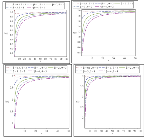
The behavior of $h (x)$ of WGD for different combinations of $θ$ and $β$ are shown in Figure 3.

Figure 3 Behavior of the hazard function of WGD for different combinations

$θ$ and

$β .$

Mean residual life function

The mean residual life function $μ (x) = E (X - x | X > x)$ of the WGD can be derived as

$μ (x) = \frac{1}{S (x; θ, β)} \int_{x}^{\infty} t f_{3} (t; θ, β) d t - x$

$= \frac{{(θ x)}^{β} (θ + β + 2) e^{- θ x} + {β^{2} + β θ + 2 β - θ x (θ + β + 1)} Γ (β, θ x)}{θ {{(θ x)}^{β} e^{- θ x} + (θ + β + 1) Γ (β, θ x)}}$

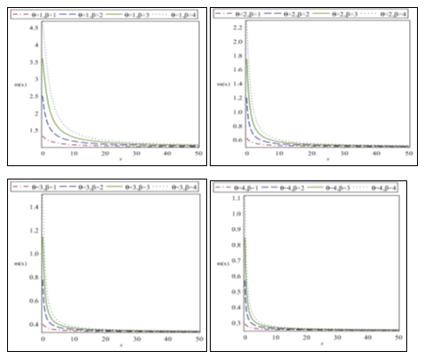
Clearly $μ (0) = \frac{β (θ + β + 2)}{θ (θ + β + 1)} = {μ^{'}}_{1}$ . The behavior of $μ (x)$ of the WGD for different combinations of $θ$ and $β$ are shown in Figure 4.

Figure 4 Behavior of

$μ (x)$ of the WGD for different cpmbinations of

$θ$ and

$β .$

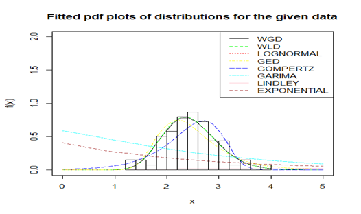
Figure 5 Fitted pdf plots of considered distribution for the given dataset.

c. Stochastic ordering

A random variable $X$ is said to be smaller than a random variable $Y$ in the

Stochastic order $(X \leq_{s t} Y)$ if $F_{X} (x) \geq F_{Y} (x)$ for all x
Hazard rate order $(X \leq_{h r} Y)$ if $h_{X} (x) \geq h_{Y} (x)$ for all x
Mean residual life order $(X \leq_{m r l} Y)$ if $m_{X} (x) \leq m_{Y} (x)$ for all x
Likelihood ratio order $(X \leq_{l r} Y)$ if $\frac{f_{X} (x)}{f_{Y} (x)}$ decreases in x.

The following important interpretations due to Shaked & Shanthikumar¹³ are well known for establishing stochastic ordering of distributions.

$\begin{array}{l} X \leq_{l r} Y \Rightarrow X \leq_{h r} Y \Rightarrow X \leq_{m r l} Y \\ ⇓ \\ X \leq_{s t} Y \end{array}$

The WGD is ordered with respect to the strongest ‘likelihood ratio’ ordering as established in the following theorem.

Theorem

Let $X ~ WGD (θ_{1}, β_{1})$ and $Y ~ WGD (θ_{2}, β_{2})$ . If $θ_{1} > θ_{2}$ and $β_{1} = β_{2}$ $(or β_{1} < β_{2} and θ_{1} = θ_{2})$ , then $X \leq_{l r} Y$ and thus $X \leq_{h r} Y$ , $X \leq_{m r l} Y$ and $X \leq_{s t} Y$ .

Proof

We have

$\ln \frac{f_{X} (x; θ_{1}, β_{1})}{f_{Y} (x; θ_{2,} β_{2})} = \ln (\frac{θ_{1}^{β_{1}} (θ_{2} + β_{2} + 1) Γ (β_{2})}{θ_{2}^{β_{2}} (θ_{1} + β_{1} + 1) Γ (β_{1})}) x^{β_{_{1}} - β_{2}} (\frac{1 + θ_{1} + θ_{1} x}{1 + θ_{2} + θ_{2} x}) e - (θ_{1} - θ_{2}) x$

Now $\ln \frac{f_{X} (x; θ_{1}, β_{1})}{f_{Y} (x; θ_{2,} β_{2})} = \ln (\frac{θ_{1}^{β_{1}} (θ_{2} + β_{2} + 1) Γ (β_{2})}{θ_{2}^{β_{2}} (θ_{1} + β_{1} + 1) Γ (β_{1})}) + (β_{1} - β_{2}) \ln x + \ln (\frac{1 + θ_{1} + θ_{1} x}{1 + θ_{2} + θ_{2} x}) - (θ_{1} - θ_{2}) x$

This gives

$\frac{d}{d x} \ln (\frac{f_{X} (x; θ_{1}, β_{1})}{f_{Y} (x; θ_{2}, β_{2})}) = \frac{β_{1} - β_{2}}{x} + \frac{θ_{1} - θ_{2}}{(1 + θ_{1} + θ_{1} x) (1 + θ_{2} + θ_{2} x)} - (θ_{1} - θ_{2}) .$

Thus, for $β_{1} = β_{2}$ and $θ_{1} \geq θ_{2}$ , or $(β_{1} < β_{2} and θ_{1} \geq θ_{2})$ , $\frac{d}{d x} \ln (\frac{f_{x} (x; θ_{1}, β_{1})}{f_{y} (x; θ_{2}, β_{2})}) < 0$ . This shows that $X \leq_{l r} Y$ and thus $X \leq_{h r} Y$ , $X \leq_{m r l} Y$ and $X \leq_{s t} Y$ . This shows flexibility of WGD over Garima distribution.

Estimation of parameters

Consider $(x_{1}, x_{2}, . . ., x_{n})$ be a random sample of size n from WGD (2.2). The natural log likelihood function can be expressed as

$\ln L = n [β \ln θ - \ln (θ + β + 1) - \ln (Γ (β))] + (β - 1) \sum_{i = 1}^{n} \ln (x_{i}) + \sum_{i = 1}^{n} \ln (1 + θ + θ x_{i}) - n θ \bar{x}$

The maximum likelihood estimates ( $\hat{θ}$ , $\overset{⌢}{β}$ ) of $(θ, β)$ is the solution of the following log likelihood equations.

$\frac{\partial \ln L}{\partial θ} = \frac{n β}{θ} - \frac{n}{θ + β + 1} + \sum_{i = 1}^{n} \frac{1 + x_{i}}{1 + θ + θ x_{i}} - n \bar{x} = 0$

$\frac{\partial \ln L}{\partial β} = n \ln θ - \frac{n}{θ + β + 1} - n ψ (β) + \sum_{i = 1}^{n} \ln (x_{i}) = 0$

where $\bar{x}$ being the sample mean and $ψ (β)$ is the digamma function defined as $ψ (β) = \frac{d}{d β} \ln Γ (β)$ . Since these two log likelihood equations are not in closed forms, they cannot be solved analytically. However, the MLE’s $(\hat{θ}, \hat{β})$ of $(θ, β)$ can be computed directly by solving the natural log likelihood equation using Newton–Raphson method available in R–software till sufficiently close estimates of $\overset{⌢}{θ}$ and $\overset{⌢}{β}$ are obtained. In this paper starting values of parameters $θ$ and $β$ are $θ = 0.5$ and $β = 1.5$ , respectively.

Data analysis

In this section a real lifetime data has been considered for the goodness of fit of WGD over one–parameter and two–parameter life time distributions. The data is regarding the tensile strength, measured in GPa, of 69 carbon fibers tested under tension at gauge lengths of 20mm, available in Bader & Priest.¹⁴

1.312 1.314 1.479 1.552 1.700 1.803 1.861 1.865 1.944 1.958 1.966 1.997 2.006 2.021 2.027 2.055 2.063 2.098 2.140 2.179 2.224 2.240 2.253 2.270 2.272 2.274 2.301 2.301 2.359 2.382 2.382 2.426 2.434 2.435 2.478 2.490 2.511 2.514 2.535 2.554 2.566 2.570 2.586 2.629 2.633 2.642 2.648 2.684 2.697 2.726 2.770 2.773 2.800 2.809 2.818 2.821 2.848 2.880 2.954 3.012 3.067 3.084 3.090 3.096 3.128 3.233 3.433 3.585 3.585

The goodness of fit of WGD has been compared with one parameter exponential, Lindley and Garima distributions and two–parameter Gompertz distribution, generalized exponential distribution (GED) introduced by Gupta & Kundu¹⁵, lognormal distribution and WLD. The pdf and cdf of Gompertz distributions, lognormal and GED are presented in Table 5. The ML estimates of parameters, $- 2 \ln L$ , Akaike Information criteria (AIC), K–S statistics and p–value of distributions for the considered dataset are presented in Table 6. The AIC and K–S Statistics are calculated using the formulae: $A I C = - 2 \ln L + 2 k$ and $K-S = \underset{x}{Sup} | F_{n} (x) - F_{0} (x) |$ , where $k$ = the number of parameters, n = the sample size, $F_{n} (x)$ is the empirical (sample) cumulative distribution function, and $F_{0} (x)$ is the theoretical cumulative distribution function. The best distribution is the distribution corresponding to lower values of $- 2 \ln L$ , AIC, and K–S statistics.

It is quite obvious from table 6 that WGD is competing well with two–parameter lifetime distributions and gives quite satisfactory fit.

Distributions	pdf	cdf
WLD	$f (x; θ, β) = \frac{θ^{β + 1}}{(θ + β)} \frac{x^{β - 1}}{Γ (β)} (1 + x) e^{- θ x}$	$F (x; θ, β) = 1 - \frac{(θ + β) Γ (β, θ x) + {(θ x)}^{β} e^{- θ x}}{(θ + β) Γ (β)}$
Lognormal	$f (x; θ, β) = \frac{1}{\sqrt{2 π} β x} e^{- \frac{1}{2} {(\frac{\log x - θ}{β})}^{2}}$	$F (x; θ, β) = ϕ (\frac{\log x - θ}{β})$
GED	$f (x; θ, β) = θ β {(1 - e^{- θ x})}^{β - 1} e^{- θ x}$	$F (x; θ, β) = {(1 - e^{- θ x})}^{β}$
Gompertz	$f (x; θ, β) = θ e^{β x - \frac{θ}{β} (e^{β x} - 1)}$	$F (x; θ, β) = 1 - e^{- \frac{θ}{β} (e^{β x} - 1)}$

Table 5 The pdf and the cdf of fitted distributions

Distributions	ML Estimates		$- 2 \ln L$	AIC	K-S	P-value
Distributions	$\hat{θ}$	$β$	$- 2 \ln L$	AIC	K-S	P-value
WGD	9.3798	22.3473	101.94	105.94	0.057	0.979
WLD	9.6265	22.8938	101.95	105.95	0.059	0.973
Lognormal	0.8751	0.2124	102.72	106.73	0.103	0.713
GED	2.0331	87.2847	109.24	113.24	0.087	0.613
Gompertz	0.0080	2.0420	107.25	111.250	0.085	0.673
Garima	0.5863	-------	251.33	253.33	0.4381	0.000
Lindley	0.0702	-------	238.38	240.38	0.401	0.000
Exponential	0.4079	-------	261.73	263.73	0.448	0.000

Table 6 MLE’s, - 2ln L, AIC, K-S Statistics and p-values of the fitted distributions

Conclusion

A two–parameter weighted Garima distribution(WGD) which includes one parameter Garima distribution proposed by Shanker⁵ has been suggested for modeling lifetime data from engineering. Its statistical properties including shapes of probability density function for different combinations of parameters, coefficients of variation, skweness, kurtosis, and index of dispersion have been explained. Reliability measures including hazard rate function, mean residual life function and the stochastic ordering have been studied. Estimation of parameters has been discussed using maximum likelihood. The goodness of fit of WGD has been explained with a real lifetime data and the fit has been found to be quite satisfactory over exponential, Lindley and Garima, Gompertz, generalized exponential, lognormal and weighted Lindley distributions.

References

- Fisher RA. The effects of methods of ascertainment upon the estimation of frequencies. Ann Eugenics. 1934;6(1):13–25.
- Rao CR. On discrete distributions arising out of methods of ascertainment. In: Patil GP, editor. Classical and Contagious Discrete Distributions. Calcutta: Statistical Publishing Society; 1965. p. 320–332.
- Patil GP, Rao CR. The Weighted distributions: A survey and their applications. In applications of Statistics. PR Krishnaiah, editor. Amsterdam: North Holland Publications Co; 1977. p. 383–405,
- Patil GP, Rao CR. Weighted distributions and size-biased sampling with applications to wild-life populations and human families. Biometrics. 1978;34:179–189.
- Shanker R. Garima distribution and Its Application to model behavioral science data. Biometrics & Biostatistics International Journal. 2016;4(7):1–9.
- Lindley DV. Fiducial distributions and Bayes’theorem. Journal of the Royal Statistical Society. Series B. 1958;20(1):102–107.
- Ghitany ME, Atieh B, Nadarajah S. Lindley distribution and its Application. Mathematics Computing and Simulation. 2008;78(4):493–506.
- Ghitany ME, Alqallaf F, Al-Mutairi DK, et al. A two-parameter weighted Lindley distribution and its applications to survival data. Mathematics and Computers in simulation. 2011;81(6):1190–1201.
- Shanker R, Shukla KK, Mishra A. A three-parameter weighted Lindley distribution. Statistics in Transition new series. 2017;18(2):291–300.
- Shanker R. The discrete Poisson-Garima distribution. Biometrics and Biostatistics International Journal. 2017;5(2):1–7.
- Shanker R, Shukla KK. Size-biased Poisson-Garima distribution with applications. Biometrics and Biostatistics International Journal. 2017;6(3):1-6.
- Shanker R, Shukla KK. Zero-truncated Poisson-Garima distribution with applications. Biometrics and Biostatistics Open Access Journal. 2017 b;3(1):1-6.
- Shaked M, Shanthikumar JG. Stochastic Orders and Their Applications. New York: Academic Press; 1994.
- Bader MG, Priest AM. Statistical aspects of fiber and bundle strength in hybrid composites. In; hayashi T, Kawata K, Umekawa S. editors, ICCM-IV, Tokyo: Progress in Science in Engineering Composites; 1982. p. 1129–1136.
- Gupta RD, Kundu D. Generalized exponential distribution. Australian and Newzealand Journal of statistics. 1999;41(2):173–188.
©2018 Eyob, et al. This is an open access article distributed under the terms of the,
which
permits unrestricted use, distribution, and build upon your work non-commercially.