In this paper, a weighted Pratibha distribution introduced to modelling life time data using the weighted transformation technique in Pratibha distribution. Its statistical properties including survival function, hazard function, reverse hazard function, mean residual life function stochastic ordering, moments related measures such as moments about origin, moments about mean, coefficient of variation, skewness, kurtosis, index of dispersion have been studied. Parameters are estimated by method of maximum likelihood estimation. A simulation study has been carried out to test the consistency of the parameters obtained through the maximum likelihood method. The goodness of fit of the distribution has been presented with a real lifetime dataset and the goodness of fit shows better fit over weighted Sujatha distribution, weighted Komal distribution, weighted Lindley distribution, weighted Garima distribution and weighted Aradhana distribution.

Keywords: Pratibha distribution, statistical properties, maximum likelihood estimation, simulation, application

Fisher¹ initially developed the concept of weighted distributions to represent the ascertainment bias. Subsequently, Rao² extended this idea cohesively while modelling statistical data in which standard distributions were not appropriate for recording these observations with equal probability. To capture the observations in such instances’, weighted models were created using a weighted function. Biased data will arise from the frequency distribution of data recorded such as at least one boy child per family, at least one girl child per family, at least one migration per family, etc.

Assume that the original observation y is based on a distribution with probability density function (pdf) $g_y\left(x,{\eta }_1\right)$ , where ${\eta }_1$  may be a vector of parameters and that the observation x is recorded based on a probability that is re-weighted by weight function $w\left(x,{\eta }_2\right)>0$ , where ${\eta }_2$  is a new parameter vector.

$f\left(x;{\eta }_1,{\eta }_2\right)=Dw\left(x;{\eta }_2\right)g_y\left(x;{\eta }_1\right)$

where D is a constant used to normalize. Note that these kinds of distributions are referred to as weighted distributions. The simple size-biased distributions or length-biased distributions are the weighted distributions with the weight function $w\left(x\right)=x$ . A few broad probability models that produce weighted probability distributions were examined by Patil³ and Rao,⁴ along with applications and the fact that $w\left(x\right)=x$ is a natural outcome in sampling-related situations.

In distribution theory, it is highly helpful to add a shape parameter to an existing distribution using a weighted approach. The existing distribution exhibits increased flexibility and tractability tendencies with the inclusion of a parameter. Weighted distributions are used to model heterogeneity, clustered sampling, and extraneous variance in the dataset.

Weighted versions of one parameter lifetime distributions have been derived by several researchers using the weight function $w\left(x,\omega \right)=x^{\omega -1}$ . For examples, Ghitany et al.⁵ proposed weighted Lindley distribution (WLD) from Lindley distribution of Lindley,⁶ Eyob and Shanker⁷ suggested weighted Garima distribution (WGD) from Garima distributions of Shanker,⁸ Ganaie et al.⁹ suggested weighted Aradhana distribution (WAD) from Aradhana distribution of Shanker,¹⁰ Shanker and Shukla¹¹ suggested weighted Sujatha distribution (WSD) from Sujatha distribution of Shanker,¹² Shanker et al.¹³ suggested weighted Komal distribution (WKD) from Komal distribution of Shanker,¹⁵ Shanker et al.¹⁴ suggested weighted Uma distribution (WUD) from Uma distribution of Shanker¹⁷ respectively. It has been noted that, depending on a conceptual or applied angle, these weighted distributions did not provide a suitable fit in certain datasets. Therefore, search for better weighted distribution corresponding to recent lifetime distribution is required.

Shanker¹⁶ introduced a one parameter Pratibha distribution with statistical properties and applications and observed that Pratibha distribution provides better fit than exponential distribution, Lindley distribution, Sujatha distribution, Shanker distribution by Shanker,¹⁸ Akash distribution by Shanker¹⁹ and Garima distribution. The pdf and cdf of Pratibha distribution are given by

$\begin{array}{l}f\left(x;\eta \right)=\frac{{\eta }^3}{\left[{\eta }^3+\eta +2\right]}\left(\eta +x+x^2\right)e^{-\eta x};x>0,\eta >0\\ F\left(x;\eta \right)=1-\left[1+\frac{\eta x\left(\eta x+\eta +2\right)}{{\eta }^3+\eta +2}\right]e^{-\eta x};x>0,\eta >0\end{array}$

The primary goal is to study the weighted Pratibha distribution (WPD) and examine its properties. The WPD is being proposed because it is expected to provide a better fit than the weighted counterpart of the Lindley, Sujatha, Komal, and Garima distributions, given that the Pratibha distribution provides the highest degree of fit over these distributions.

Weighted Pratibha distribution

Let a random variable $X~$ WPD $\left(\eta ,\omega \right)$  with the weight function $w\left(x,\omega \right)=x^{\omega -1}$ , the pdf and cdf of WPD can be expressed as

$\begin{array}{l}f\left(x;\eta ,\omega \right)=\frac{{\eta }^{\omega +2}}{\left[{\eta }^3+\eta \omega +\omega \left(\omega +1\right)\right]\Gamma \left(\omega \right)}\left(\eta +x+x^2\right)x^{\omega -1}{e}^{-\eta x};x>0,\eta >0,\omega >0\\ F\left(x;\eta ,\omega \right)=1-\frac{{\eta }^3\Gamma \left(\omega ,\eta x\right)+\eta \Gamma \left(\omega +1,\eta x\right)+\Gamma \left(\omega +2,\eta x\right)}{\left[{\eta }^3+\eta \omega +\omega \left(\omega +1\right)\right]\Gamma \left(\omega \right)};x>0,\eta >0,\omega >0\end{array}$

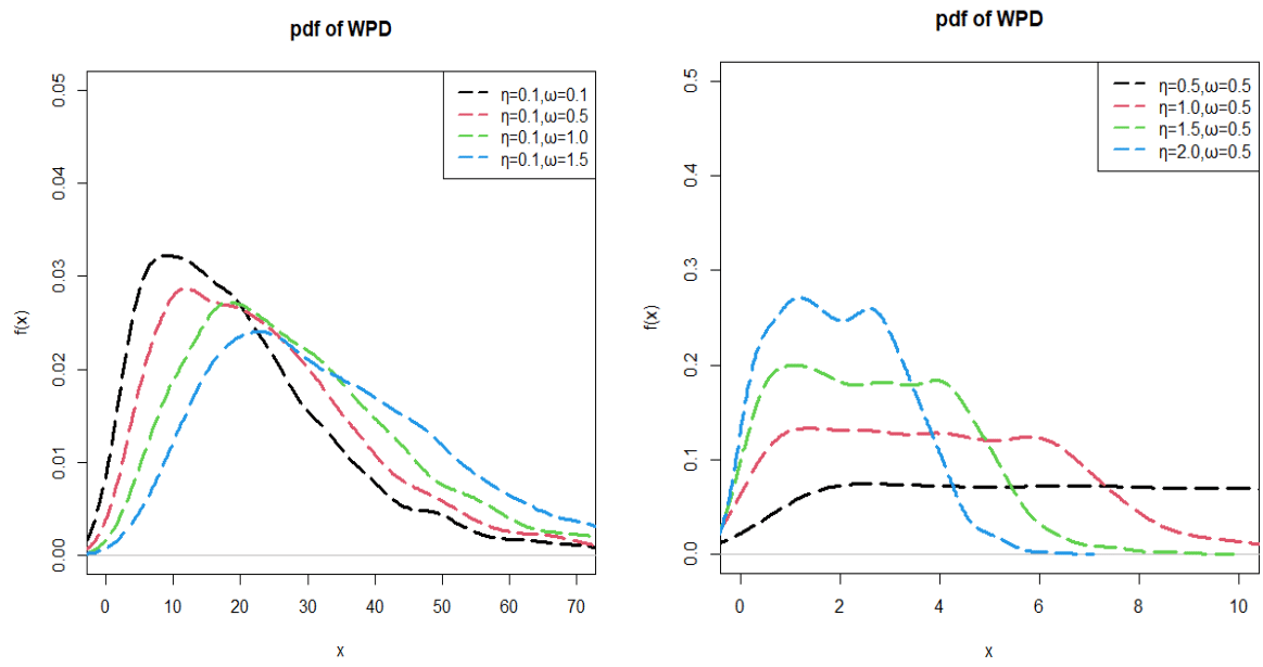
where $\eta$ is a scale parameter and $\omega$  is shape parameter of the distribution. When $\omega =1$ , WPD reduced to Pratibha distribution with parameter $\eta$ . The plots of pdf and cdf of WPD are shown in the following Figures 1 & 2 respectively. From the Figure 1, it is clear that when $\eta =0.1$  and for increasing values of $\omega$ , the pdf has unimodal and positively skeweed natures. When $\omega =0.5$  and $\eta <0.1$ , it has monotonically increasing natures and for $\omega =0.5$  and $\eta \ge 1$ , the pdf have bimodal and positively skewwed natures. The most important feature of WPD is that it is unimodal and bimodal for different values of parameters and in general flood dataset shows unimodal or bimodal shapes depending upon the time period of the flood and WPD would be the best choice for modeling data of flood.

Figure 1 pdf of WPD.

Figure 2 cdf of WPD.

Survival function

The survival function of WPD can be obtained as

$S\left(x;\eta ,\omega \right)=\frac{{\eta }^3\Gamma \left(\omega ,\eta x\right)+\eta \Gamma \left(\omega +1,\eta x\right)+\Gamma \left(\omega +2,\eta x\right)}{\left[{\eta }^3+\eta \omega +\omega \left(\omega +1\right)\right]\Gamma \left(\omega \right)};x>0,\eta >0,\omega >0$

Hazard function

The hazard function of WPD can be obtained as

$h\left(x;\eta ,\omega \right)=\frac{{\eta }^{\omega +2}\left(\eta +x+x^2\right)x^{\omega -1}{e}^{-\eta x}}{{\eta }^3\Gamma \left(\omega ,\eta x\right)+\eta \Gamma \left(\omega +1,\eta x\right)+\Gamma \left(\omega +2,\eta x\right)};x>0,\eta >0,\omega >0$

The plots of hazard function of WPD are graphically shown in the following Figure 3. It shows different shapes including monotonically increasing, decreasing, upside bathtub and downside bathtub and it means that the distribution is applicable for modelling data of these natures.

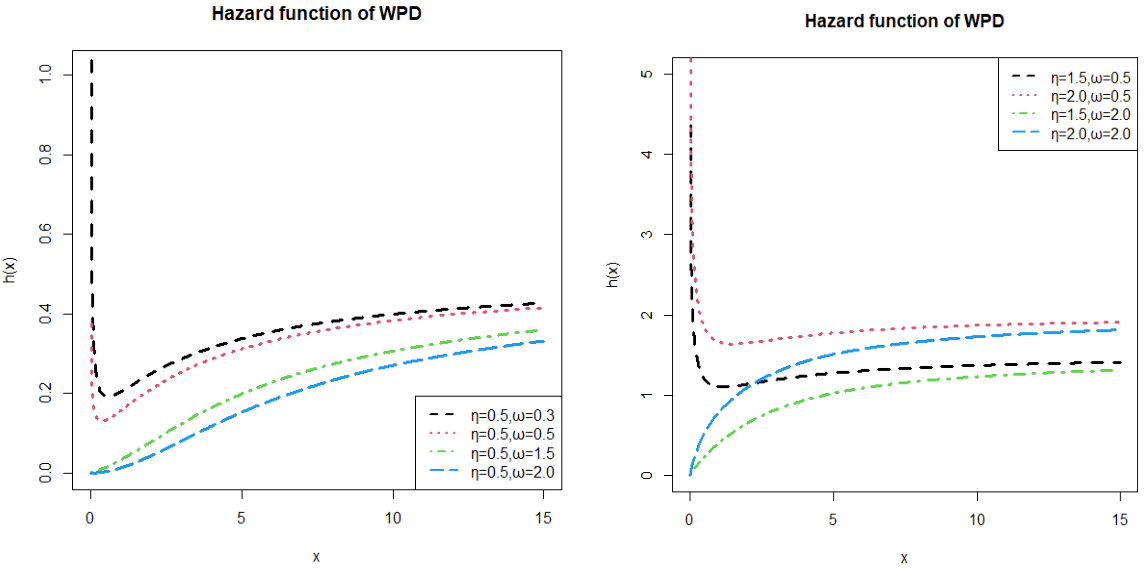
Figure 3 Hazard function of WPD.

Reverse hazard function

$r\left(x;\eta ,\omega \right)=\frac{{\eta }^{\omega +2}\left(\eta +x+x^2\right)x^{\omega -1}{e}^{-\eta x}}{\left[{\eta }^3+\eta \omega +\omega \left(\omega +1\right)\right]\Gamma \left(\omega \right)-{\eta }^3\Gamma \left(\omega ,\eta x\right)+\eta \Gamma \left(\omega +1,\eta x\right)+\Gamma \left(\omega +2,\eta x\right)};x>0,\eta >0,\omega >0$

Mean residual life function

Mean residual life function of WPD can be obtained as

$m\left(x;\eta ,\omega \right)=\frac{{\eta }^3\Gamma \left(\omega +1,\eta x\right)+\eta \Gamma \left(\omega +2,\eta x\right)+\Gamma \left(\omega +3,\eta x\right)}{\eta \left[{\eta }^3\Gamma \left(\omega ,\eta x\right)+\eta \Gamma \left(\omega +1,\eta x\right)+\Gamma \left(\omega +2,\eta x\right)\right]}-x;x>0,\eta >0,\omega >0$ .

The plots of mean residual life function are shown in the following Figure 4. It is quite obvious that mean residual life function is monotonically decreasing.

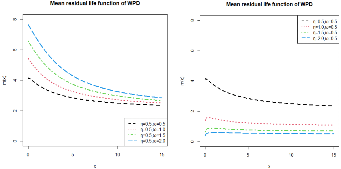
Figure 4 Mean residual life function of WPD.

Moments related measures

The rth raw moment (moment about origin) of WPD, after little algebraic simplification, can be obtained as

${\mu }_r{}^{\prime }={\displaystyle \underset{0}{\overset{\infty }{\int }}{x}^{r}f\left(x;\eta ,\omega \right)}dx=\frac{\Gamma \left(\omega +r\right)\left[{\eta }^3+\eta \left(\omega +r\right)+\left(\omega +r\right)\left(\omega +r+1\right)\right]}{{\eta }^r\left[{\eta }^3+\eta \omega +\omega \left(\omega +1\right)\right]\Gamma \left(\omega \right)};r=1,2,\mathrm{3...}$

Putting $r=1,2,3,4$ , the first four raw moments are obtained as

${\mu }_1{}^{\prime }=\frac{\omega \left[{\eta }^3+\eta \left(\omega +1\right)+\left(\omega +1\right)\left(\omega +2\right)\right]}{\eta \left[{\eta }^3+\eta \omega +\omega \left(\omega +1\right)\right]}$

${\mu }_2{}^{\prime }=\frac{\omega \left(\omega +1\right)\left[{\eta }^3+\eta \left(\omega +2\right)+\left(\omega +2\right)\left(\omega +3\right)\right]}{{\eta }^2\left[{\eta }^3+\eta \omega +\omega \left(\omega +1\right)\right]}$

${\mu }_3{}^{\prime }=\frac{\omega \left(\omega +1\right)\left(\omega +2\right)\left[{\eta }^3+\eta \left(\omega +3\right)+\left(\omega +3\right)\left(\omega +4\right)\right]}{{\eta }^3\left[{\eta }^3+\eta \omega +\omega \left(\omega +1\right)\right]}$

${\mu }_4{}^{\prime }=\frac{\omega \left(\omega +1\right)\left(\omega +2\right)\left(\omega +3\right)\left[{\eta }^3+\eta \left(\omega +4\right)+\left(\omega +4\right)\left(\omega +5\right)\right]}{{\eta }^4\left[{\eta }^3+\eta \omega +\omega \left(\omega +1\right)\right]}$

The central moments of WPD, after simple algebraic simplification, can be obtained as

${\mu }_2=\frac{\omega \left[\begin{array}{l}{\eta }^6+2{\eta }^4\omega +2{\eta }^3{\omega }^2+2{\eta }^4+8{\eta }^3\omega +{\eta }^2{\omega }^2+2\eta {\omega }^3\\ +{\omega }^4+6{\eta }^3+{\eta }^2\omega +6\eta {\omega }^2+4{\omega }^3+4\eta \omega +5{\omega }^2+2\omega \end{array}\right]}{{\eta }^2{\left({\eta }^3+\eta \omega +{\omega }^2+\omega \right)}^2}$

${\mu }_3=\frac{2\omega \left[\begin{array}{l}{\eta }^9+3{\eta }^7\omega +3{\eta }^6{\omega }^2+3{\eta }^7+15{\eta }^6\omega +3{\eta }^5{\omega }^2+\\ 6{\eta }^4{\omega }^3+3{\eta }^3{\omega }^4+12{\eta }^6+3{\eta }^5\omega +21{\eta }^4{\omega }^2\\ +13{\eta }^3{\omega }^3+3{\eta }^2{\omega }^4+3\eta {\omega }^5+{\omega }^6+15{\eta }^4\omega +\\ 16{\eta }^3{\omega }^2+9{\eta }^2{\omega }^3+12\eta {\omega }^4+5{\omega }^5+6{\eta }^3\omega \\ +6{\eta }^2{\omega }^2+15\eta {\omega }^3+9{\omega }^4+6\eta {\omega }^2+7{\omega }^3+2{\omega }^2\end{array}\right]}{{\eta }^3{\left({\eta }^3+\eta \omega +{\omega }^2+\omega \right)}^3}$

${\mu }_4=\frac{3\omega \left[\begin{array}{l}2{\eta }^{12}+{\eta }^{12}\omega +4{\eta }^{10}{\omega }^2+4{\eta }^9{\omega }^3+12{\eta }^{10}\omega +\\ 24{\eta }^9{\omega }^2+6{\eta }^8{\omega }^3+12{\eta }^7{\omega }^4+6{\eta }^6{\omega }^5+8{\eta }^{10}\\ +60{\eta }^9\omega +22{\eta }^8{\omega }^2+76{\eta }^7{\omega }^3+56{\eta }^6{\omega }^4+\\ 12{\eta }^5{\omega }^5+12{\eta }^4{\omega }^6+4{\eta }^3{\omega }^7+40{\eta }^9+16{\eta }^8\omega \\ +160{\eta }^7{\omega }^2+158{\eta }^6{\omega }^3+76{\eta }^5{\omega }^4+101{\eta }^4{\omega }^5\\ +44{\eta }^3{\omega }^6+6{\eta }^2{\omega }^7+4\eta {\omega }^8+{\omega }^9+96{\eta }^7\omega \\ +164{\eta }^6{\omega }^2+148{\eta }^5{\omega }^3+272{\eta }^4{\omega }^4+160{\eta }^3{\omega }^5\\ +46{\eta }^2{\omega }^6+36\eta {\omega }^7+10{\omega }^8+56{\eta }^6{\omega }^3\\ 84{\eta }^5{\omega }^2+287{\eta }^4{\omega }^3+252{\eta }^3{\omega }^4+118{\eta }^2{\omega }^5\\ +116\eta {\omega }^6+38{\omega }^7+104{\eta }^4{\omega }^2+172{\eta }^3{\omega }^3\\ 38{\omega }^4+8{\omega }^3\end{array}\right]}{{\eta }^4{\left({\eta }^3+\eta \omega +{\omega }^2+\omega \right)}^4}$

Thus, the coefficient of variation (C.V), coefficient of skewness $\left(\sqrt{{\beta }_1}\right)$ , coefficient of kurtosis $\left({\beta }_2\right)$ , and index of dispersion $\left(\gamma \right)$ of WPD are obtained as

$CV=\frac{\sqrt{\omega \left[\begin{array}{l}{\eta }^6+2{\eta }^4\omega +2{\eta }^3{\omega }^2+2{\eta }^4+8{\eta }^3\omega +{\eta }^2{\omega }^2+2\eta {\omega }^3\\ +{\omega }^4+6{\eta }^3+{\eta }^2\omega +6\eta {\omega }^2+4{\omega }^3+4\eta \omega +5{\omega }^2+2\omega \end{array}\right]}}{\omega \left[{\eta }^3+\eta \left(\omega +1\right)+\left(\omega +1\right)\left(\omega +2\right)\right]}$

$\sqrt{{\beta }_1}=\frac{2\omega \left[\begin{array}{l}{\eta }^9+3{\eta }^7\omega +3{\eta }^6{\omega }^2+3{\eta }^7+15{\eta }^6\omega +3{\eta }^5{\omega }^2\\ +6{\eta }^4{\omega }^3+3{\eta }^3{\omega }^4+12{\eta }^6+3{\eta }^5\omega +21{\eta }^4{\omega }^2\\ +13{\eta }^3{\omega }^3+3{\eta }^2{\omega }^4+3\eta {\omega }^5+{\omega }^6+15{\eta }^4\omega +\\ 16{\eta }^3{\omega }^2+9{\eta }^2{\omega }^3+12\eta {\omega }^4+5{\omega }^5+6{\eta }^3\omega \\ +6{\eta }^2{\omega }^2+15\eta {\omega }^3+9{\omega }^4+6\eta {\omega }^2+7{\omega }^3+2{\omega }^2\end{array}\right]}{\omega \left[\begin{array}{l}{\eta }^6+2{\eta }^4\omega +2{\eta }^3{\omega }^2+2{\eta }^4+8{\eta }^3\omega +{\eta }^2{\omega }^2+2\eta {\omega }^3\\ +{\omega }^4+6{\eta }^3+{\eta }^2\omega +6\eta {\omega }^2+4{\omega }^3+4\eta \omega +5{\omega }^2+2\omega \end{array}\right]}$

${\beta }_2=\frac{3\omega \left[\begin{array}{l}2{\eta }^{12}+{\eta }^{12}\omega +4{\eta }^{10}{\omega }^2+4{\eta }^9{\omega }^3+12{\eta }^{10}\omega +\\ 24{\eta }^9{\omega }^2+6{\eta }^8{\omega }^3+12{\eta }^7{\omega }^4+6{\eta }^6{\omega }^5+8{\eta }^{10}\\ +60{\eta }^9\omega +22{\eta }^8{\omega }^2+76{\eta }^7{\omega }^3+56{\eta }^6{\omega }^4+\\ 12{\eta }^5{\omega }^5+12{\eta }^4{\omega }^6+4{\eta }^3{\omega }^7+40{\eta }^9+16{\eta }^8\omega \\ +160{\eta }^7{\omega }^2+158{\eta }^6{\omega }^3+76{\eta }^5{\omega }^4+101{\eta }^4{\omega }^5\\ +44{\eta }^3{\omega }^6+6{\eta }^2{\omega }^7+4\eta {\omega }^8+{\omega }^9+96{\eta }^7\omega \\ +164{\eta }^6{\omega }^2+148{\eta }^5{\omega }^3+272{\eta }^4{\omega }^4+160{\eta }^3{\omega }^5\\ +46{\eta }^2{\omega }^6+36\eta {\omega }^7+10{\omega }^8+56{\eta }^6{\omega }^3\\ 84{\eta }^5{\omega }^2+287{\eta }^4{\omega }^3+252{\eta }^3{\omega }^4+118{\eta }^2{\omega }^5\\ +116\eta {\omega }^6+38{\omega }^7+104{\eta }^4{\omega }^2+172{\eta }^3{\omega }^3\\ 38{\omega }^4+8{\omega }^3\end{array}\right]}{{\omega }^2{\left[\begin{array}{l}{\eta }^6+2{\eta }^4\omega +2{\eta }^3{\omega }^2+2{\eta }^4+8{\eta }^3\omega +{\eta }^2{\omega }^2+2\eta {\omega }^3\\ +{\omega }^4+6{\eta }^3+{\eta }^2\omega +6\eta {\omega }^2+4{\omega }^3+4\eta \omega +5{\omega }^2+2\omega \end{array}\right]}^2}$

$\gamma =\frac{\omega \left[\begin{array}{l}{\eta }^6+2{\eta }^4\omega +2{\eta }^3{\omega }^2+2{\eta }^4+8{\eta }^3\omega +{\eta }^2{\omega }^2+2\eta {\omega }^3\\ +{\omega }^4+6{\eta }^3+{\eta }^2\omega +6\eta {\omega }^2+4{\omega }^3+4\eta \omega +5{\omega }^2+2\omega \end{array}\right]}{\omega \eta \left({\eta }^3+\eta \omega +{\omega }^2+\omega \right)\left[{\eta }^3+\eta \left(\omega +1\right)+\left(\omega +1\right)\left(\omega +2\right)\right]}$

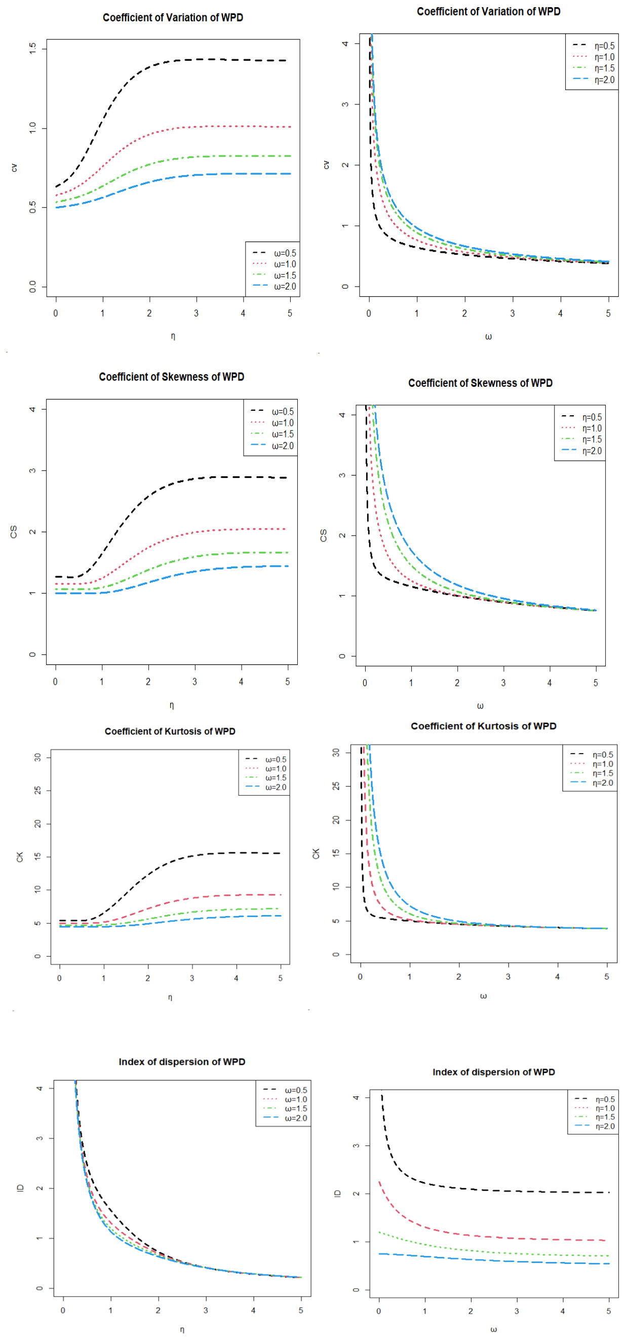
When $\eta \le 1.3,\omega \le 1.3$ , variance is greater than the mean. The plots of coefficient of variation, skewness, kurtosis and index of dispersion are shown in the following Figure 5.

Figure 5 Coefficient of variation, coefficient of skewness, coefficient of kurtosis, index of dispersion for differnet values of the parameters of WPD.

Figure 5 illustrates that for fixed values of ω and increasing values of η, the coefficient of variation, coefficient of skewness and coefficient of kurtosis are monotonically increaseing, wheres as for fixed values of η and increasing values of ω, coefficient of variation, coefficient of skewness and coefficient of kurtosis are monotonically decreaseing. On the other hand for fixed values of ω and increasing values of η and ficxed values η and incrasing values of ω index of dispersion is decreasing.

Maximum likelihood estimation

Let $\left(x_{{}_1},x_{{}_2},\mathrm{...},x_{{}_n}\right)$ be a random sample from WPD. The log-likelihood function of WPD can be expressed as

$\begin{array}{l}\log L=n\left[\left(\omega +2\right)\log \eta -\log \left({\eta }^3+\eta \omega +\omega \left(\omega +1\right)\right)\right]-n\log \left(\Gamma \left(\omega \right)\right)\\ +{\displaystyle \sum _{i=1}^n\log \left(\eta +x_i+\text{}\text{}{x}_i{}^2\right)}+\left(\omega -1\right){\displaystyle \sum _{i=1}^n\log \left(x_i\right)}-\eta {\displaystyle \sum _{i=1}^n{x}_i}\end{array}$

This gives

$\frac{\partial \log L}{\partial \eta }=\frac{n\left(\omega +2\right)}{\eta }-\frac{n\left(3{\eta }^2+\omega \right)}{{\eta }^3+\eta \omega +\omega \left(\omega +1\right)}+{\displaystyle \sum _{i=1}^n\frac{1}{\eta +x_i+x_i{}^2}}-{\displaystyle \sum _{i=1}^n{x}_i=0}$

$\frac{\partial \log L}{\partial \omega }=n\log \left(\eta \right)-\frac{n\left(\eta +2\omega +1\right)}{{\eta }^3+\eta \omega +\omega \left(\omega +1\right)}-n\psi \left(\omega \right)+{\displaystyle \sum _{i=1}^n\log x_i}=0$

where $\psi \left(\omega \right)=\frac{\partial }{\partial \omega }\log \left(\Gamma \left(\omega \right)\right)$  is a digamma function.

The log-likelihood equations presented here are not readily solvable in closed form, necessitating the use of maximization techniques using R software. Iterative solutions are employed to optimize the likelihood function until sufficiently close parameter values are achieved. These equations can be solved using Fisher’s scoring method. For Fisher's scoring method, the following approach is undertaken

$\frac{{\partial }^2\log L}{\partial {\eta }^2}=-\frac{n\left(\omega +2\right)}{{\eta }^2}-\frac{6n\eta \left[{\eta }^3+\eta \omega +\omega \left(\omega +1\right)\right]-n{\left(3{\eta }^2+\omega \right)}^2}{{\left[{\eta }^3+\eta \omega +\omega \left(\omega +1\right)\right]}^2}-{\displaystyle \sum _{i=1}^n\frac{1}{{\left(\eta +x_i+x_i{}^2\right)}^2}}$

$\frac{{\partial }^2\log L}{\partial {\omega }^2}=-\frac{2n\left[{\eta }^3+\eta \omega +\omega \left(\omega +1\right)\right]-n{\left(\eta +2\omega +1\right)}^2}{{\left[{\eta }^3+\eta \omega +\omega \left(\omega +1\right)\right]}^2}-n{\psi }^{\prime }\left(\omega \right)$

$\frac{{\partial }^2\log L}{\partial \eta \partial \omega }=-\frac{n}{\eta }-\frac{6n\eta \left[{\eta }^3+\eta \omega +\omega \left(\omega +1\right)\right]-n\left(\eta +2\omega +1\right)\left(3{\eta }^2+\omega \right)}{{\left[{\eta }^3+\eta \omega +\omega \left(\omega +1\right)\right]}^2}=\frac{{\partial }^2\log L}{\partial \omega \partial \eta }$

For finding the MLEs $\left(\widehat{\eta },\widehat{\omega }\right)$  of parameters $\left(\eta ,\omega \right)$  of WPD, following equations can be solved

${\left(\begin{array}{cc}\frac{{\partial }^2\log L}{\partial {\eta }^2}& \frac{{\partial }^2\log L}{\partial \eta \partial \omega }\\ \frac{{\partial }^2\log L}{\partial \omega \partial \eta }& \frac{{\partial }^2\log L}{\partial {\omega }^2}\end{array}\right)}_{\begin{array}{l}\widehat{\eta }={\eta }_0\\ \widehat{\omega }={\omega }_0\end{array}}\left(\begin{array}{l}\widehat{\eta }-{\eta }_0\\ \widehat{\omega }-{\omega }_0\end{array}\right)=\left(\begin{array}{l}\frac{\partial \log L}{\partial \eta }\\ \frac{\partial \log L}{\partial \omega }\end{array}\right)$

where ${\eta }_0$  and ${\omega }_0$ are the initial values of $\eta$  and $\omega$ . These equations are solved iteratively till close estimates of parameters are obtained.

A simulation study

To assess the effectiveness of maximum likelihood estimators for WPD, a simulation study has been conducted. The investigation involved examining mean estimates, biases (B), mean square errors (MSEs), and variances of the maximum likelihood estimates (MLEs) for WPD, utilizing the specified formulas.

$Mean=\frac{1}{n}{\displaystyle \sum _{i=1}^n{\widehat{H}}_i},\text{}B=\frac{1}{n}{\displaystyle \sum _{i=1}^n\left({\widehat{H}}_i-H\right)},MSE=\frac{1}{n}{{\displaystyle \sum _{i=1}^n\left({\widehat{H}}_i-H\right)}}^2,Variance=MSE-B^2$ ,

where $H=\left(\eta ,\omega \right)$ and ${\widehat{H}}_i=\left({\widehat{\eta }}_i,{\widehat{\omega }}_i\right)$ .

The acceptance-rejection method of simulation study has been employed to generate data. This method is commonly used in simulation studies to produce random samples from a target distribution. The method for generating random samples from the WPD involves the following steps:

1. Generate Y from exponential $\left(\eta \right)$ distribution
2. Generates U from Uniform $\left(0,1\right)$ distribution
3. If $U\le \frac{f(y)}{Mg(y)}$ , then set $X=Y$ (“accept the sample”); otherwise (“reject the sample”) and if reject then repeat the process: step (a-c) until getting the required samples. Where $M$ is a constant
4. Each sample size is replicated 10000 times

The biases, MSEs, and variances of the MLEs of the parameters decrease for increasing sample size as evident in Tables 1 & 2. This supports the first-order asymptotic theory of MLEs.

Variance-Covariance matrix for the prameters $\eta =0.1,\omega =1.5$   and $\eta =0.2,\omega =0.3$   respectively as

$\begin{array}{l} \eta \omega \\ \begin{array}{c}\eta \\ \omega \end{array}\left(\begin{array}{cc}0.000003& 0.000005\\ 0.000005& 0.000193\end{array}\right)\end{array}$   and  $\begin{array}{l} \eta \omega \\ \begin{array}{c}\eta \\ \omega \end{array}\left(\begin{array}{cc}0.000009& 0.000001\\ 0.000001& 0.000100\end{array}\right)\end{array}$

To test the goodness of fit of WPD , we have considered a real lifetime dataset from flood discharge. The following right-skewed dataset discussed by Montfort,²⁰ presents the maximum annual flood discharges of the North Saskatchewan in units of 1000 cubic feet per second of the north Saskatchewan river at Edmonton over a period of 47 years.

19.885, 20.940, 21.820, 23.700, 24.888, 25.460, 25.760, 26.720, 27.500, 28.100, 28.600,

30.200, 30.380, 31.500, 32.600, 32.680, 34.400, 35.347, 35.700, 38.100, 39.020, 39.200,

40.000, 40.400, 40.400, 42.250, 44.020, 44.730, 44.900, 46.300, 50.330, 51.442, 57.220,

58.700, 58.800, 61.200, 61.740, 65.440, 65.597, 66.000, 74.100, 75.800, 84.100, 106.600,

109.700, 121.970, 121.970, 185.560.

The summary of the dataset and its total time in test (TTT) plots are shown in the folowing Table 3 and the Figure 6. The goodness of fit of the WPD along with other weighted and unweighted distributions are shown in the Table 4.

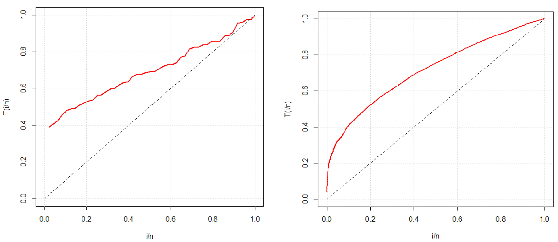
Figure 6 TTT- plot of the observed and simulated samples of WPD respectively.

The Table-4 shows that WPD have the least, AIC and K-S values as compared to the WSD, WKD, WLD, WGD, and WAD. So, we conclude that WPD provides a better fit as compared to WSD, WKD, WLD, WGD, and WAD. From the fitted plot and the P-P plot of the considered distribution presented in the Figure 7 & 8 for the dataset also exhibit that WPD provides a better fit as compared to the considered distributions.

Figure 7 Fitted plot of the considered distributions of the dataset.

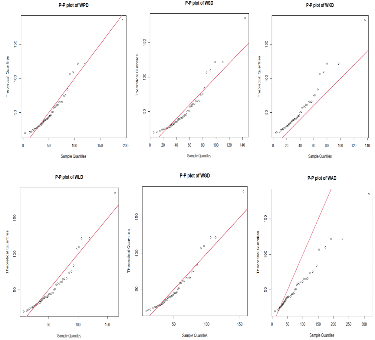
Figure 8 P-P plots of the theoretical and sample quantiles of the considered distributions of the dataset.

In this study a weighted version of Pratibha distribution known as weighted Pratibha distribution (WPD) has been proposed and discussed. Its significant statistical properties such as moments and its related measures, survival function, hazard function, reverse hazard function, and mean residual life function are studied. Parameters of the proposed distribution are estimated using the maximum likelihood estimation. A simulation study is carried out to know the performance of the estimated parameters values. Finally, an example of lifetime dataset relating to flood is carried out for the application and goodness of fit of the proposed distribution and it has been shown that it provides better fit over weighted distributions such as WSD, WKD, WLD, WGD, and WAD. Therefore, the WPD can be considered an important weighted distribution for modelling real dataset relating to flood.

Authors are grateful to the editor in chief and the anonymous reviewer for some minor comments which improved both the quality and the presentation.

The authors declare that there are no conflicts of interest.

None.

1. Fisher R.A. The effects of methods of ascertainment upon the estimation of frequencies. The Annals of Eugenics. 1934;6:13–25.
2. Rao CR. On discrete distributions arising out of methods of ascertainment, Sankhyā: The Indian Journal of Statistics, Series A. 1965;27:311–324.
3. Rao CR, Patil GP. The Weighted distributions: a survey of their applications, Application of Statistics. 1977-78;383–405.
4. Patil GP, Rao CR. Weighted distributions and size-biased sampling with applications to wildlife populations and human families. Biometrics. 1978;34:179–189.
5. Ghitany ME, Alqallaf F, Al-Mutairi, DK, et al. A two-parameter weighted Lindley distribution and its applications to survival data. Mathematics and Computers in Simulation. 2011;81(6):1190–1201.
6. Lindley DV. Fiducial distributions and Bayes’ theorem. Journal of the Royal Statistical Society, Series B. 1958;20(1):102–107.
7. Eyob T, Shanker R. A two-parameter weighted Garima distribution with properties and application. Biom Biostat Int J.. 2018;7(3):234–242.
8. Shanker, R. Garima distribution and Its Application to model behavioural science data, Biom Biostat Int J. 2016(a);4(7):275–281.
9. Ganaie RA, Rajagopalan V, Rather AA. Weighted Aradhana distribution: properties and applications. Journal of Information and Computational Science. 2019;9(8):392–406.
10. Shanker R. Aradhana distribution and its applications. International Journal of Statistics and Applications. 2016(b);6(1):23–34.
11. Shanker R, Shukla KK. A two parameter weighted Sujatha distribution and its application to model life time data, International Journal of Mathematics and Statistics. 2018;57(3):106 –121.
12. Shanker R. Sujatha distribution and its application. Statistics in Transition New Series. 2016(c);17(3):391–410.
13. Shanker R, Ray M, Prodhani HR. Weighted Komal distribution with properties and Applications, International Journal of Statistics and Reliability Engineering. 2023;10(3):541–551.
14. Shanker R, Zakaria AFM, Prodhani HR, et al. Weighted Uma distribution with properties and applications. J XIDIAN Universit. 2023;17(10):830–846.
15. Shanker R. Komal distribution with properties and application in survival analysis. Biom Biostat Int J. 2023;12(2):40–44.
16. Shanker R. Pratibha distribution with statistical properties and application. Biom Biostat Int J. 2023;12(5):136–142.
17. Shanker R. Uma distribution with properties and applications. Biom Biostat Int J. 2022;11(5):165–169.
18. Shanker R. Shanker distribution and its applications. International Journal of Statistics and Applications. 2015(a);5(6):338–348.
19. Shanker R. Akash distribution and its application. International Journal of Probability and Statistics. 2015(b);4(3):65–75.
20. Montfort M.AJV. On testing that the distribution of extremes is of type I when type II is the alternative. Journal of Hydrology. 1970;11(4):421–427.