Research Article Volume 12 Issue 5
Pratibha distribution with properties and application
Rama Shanker
shankerrama2009@gmail.com
Department of Statistics, Assam University, Silchar, Assam, India
Correspondence: Rama Shanker, Department of Statistics, Assam University, Silchar, Assam, India
Received: August 29, 2023 | Published: September 28, 2023
Citation: Shanker R. Pratibha distribution with properties and application. Biom Biostat Int J. 2023;12(5):136-142 DOI: 10.15406/bbij.2023.12.00397
Download PDF
Abstract
As we all know that the modeling and analysis of lifetime data is very challenging due to stochastic nature of data. In this paper, a new one parameter lifetime distribution named Pratibha distribution has been suggested for modeling lifetime data. Its statistical properties, estimation of parameter and an application have been discussed. The goodness of fit of Pratibha distribution has been compared with one parameter exponential, Lindley, Garima, Komal, Akash, Sujatha and Shanker distributions and the fit shows quite satisfactory.
Keywords: lifetime distributions, statistical properties, estimation of parameter, application
Introduction
The nature of the lifetime data are, in general, stochastic in nature and the existing one parameter lifetime distributions are not providing good fit. Therefore, due to stochastic nature of data, the search for a new lifetime distribution for the modeling of lifetime data is in great demand. In recent decade, several one parameter lifetime distributions have been introduced in statistics literature. For example, Lindley distribution by Lindley,1 Shanker distribution by Shanker,2 Akash distribution by Shanker,3 Sujatha distribution by Shanker,4 Garima distribution by Shanker5 and Komal distribution by Shanker,6 some among others. Shanker et al.7 have detailed study on modeling of lifetime data using exponential and Lindley distributions and concluded that there are some datasets in which these two distributions do not provide good fit. Further, Shanker et al.8 have detailed comparative study on modeling of lifetime data using exponential, Lindley and Akash distributions and observed that Akash distribution provides much better fit than both exponential and Lindley distribution but there are some data sets in which these three distributions do not provide satisfactory fit. Then, Shanker and Hagos9 put an attempt to see the modeling of the real lifetime datasets using exponential, Lindley, Shanker and Akash distributions and observed that there are some datasets in which these distributions do not provide satisfactory fit. As we all know that flexibility and tractability are the two important characteristics of any lifetime distribution and if the existing distributions are not flexible or tractable for the given dataset, then there arise the need for new lifetime distribution. Although the general practice is to transform the data to satisfy some assumptions of the distribution so that distribution fits well, but this is not useful practice because the original nature of the dataset is being lost. Therefore, the most preferable technique is to search a new one parameter lifetime distribution which provides good fit to the given data than to modify the existing one parameter lifetime distributions.
In this paper, we propose a new one parameter lifetime distribution named Pratibha distribution which provides better fit to the lifetime data over the existing one parameter lifetime distributions. The statistical properties, estimation of parameter and application of the distribution has been discussed and presented systematically. It is hoped and expected that the proposed distribution will draw attention of researchers in data science to model lifetime data and will become most preferable distribution over the existing one parameter lifetime distributions.
Pratibha distribution
Almost all one parameter lifetime distributions have been derived using the convex combination of exponential and gamma distribution with different shape parameter. Here, an attempt has been made to derive a new lifetime distribution using convex combination of exponential and gamma distributions with different shape parameter. Taking the convex combination of exponential
distribution, gamma
distribution and gamma
distribution with respective mixing proportions
and
, a new one parameter probability density function (pdf) can be expressed as
We would call this one parameter lifetime distribution as ‘Pratibha distribution’. Since it is a convex combination of exponential and gamma distributions, it is expected to give better fit over exponential and gamma distribution and other distributions developed using convex combinations of exponential and gamma distribution. The cumulative distribution function (cdf) and survival function of Pratibha distribution can be obtained as
The behaviour of the pdf and the cdf of Pratibha distribution for varying values of parameter
have been presented in Figures 1&2 respectively. It is quite obvious that the Pratibha distribution is positively skewed and hence it can be used to model positively skewed lifetime data.
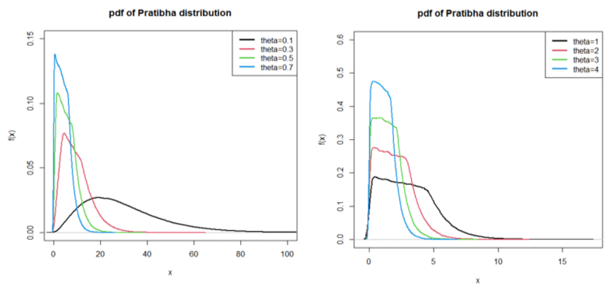
Figure 1 pdf of Pratibha distribution for selected values of the parameter.
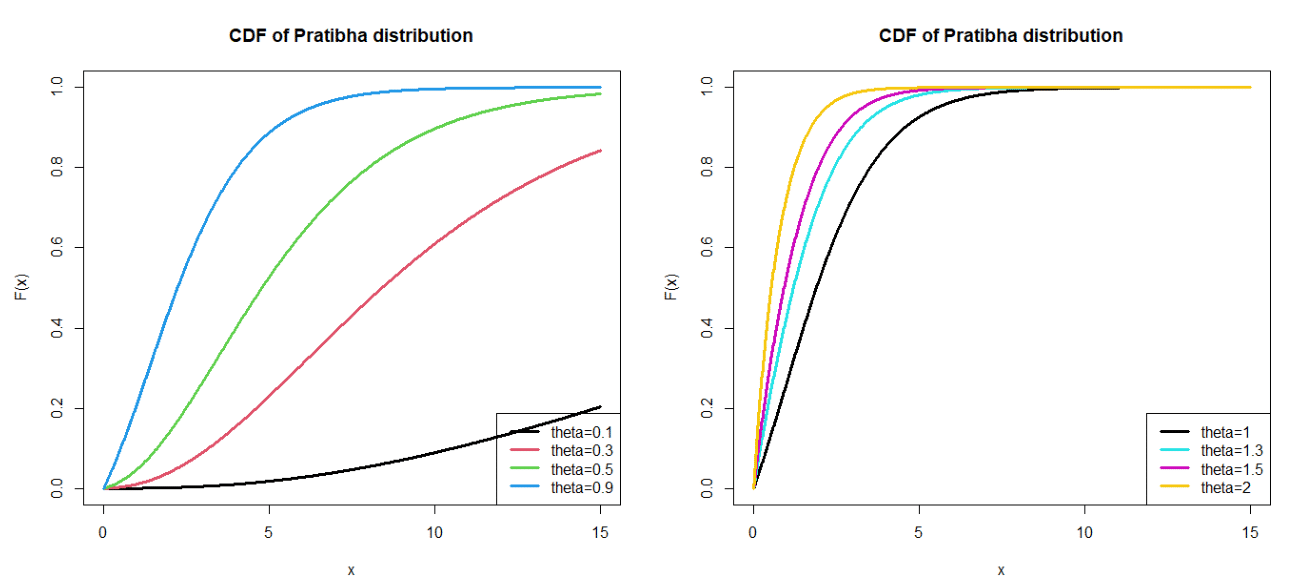
Figure 2 cdf of Pratibha distribution for selected values of the parameter.
Reliability properties
Hazard function
The hazard function of a random variable
having pdf
and cdf
is defined as
Thus, the hazard function of Pratibha distribution can be obtained as
.
This gives
. The behaviour of the hazard function of Pratibha distribution for various values of parameter
is shown in the following Figure 3. The hazard function of Pratibha distribution is monotonically increasing.
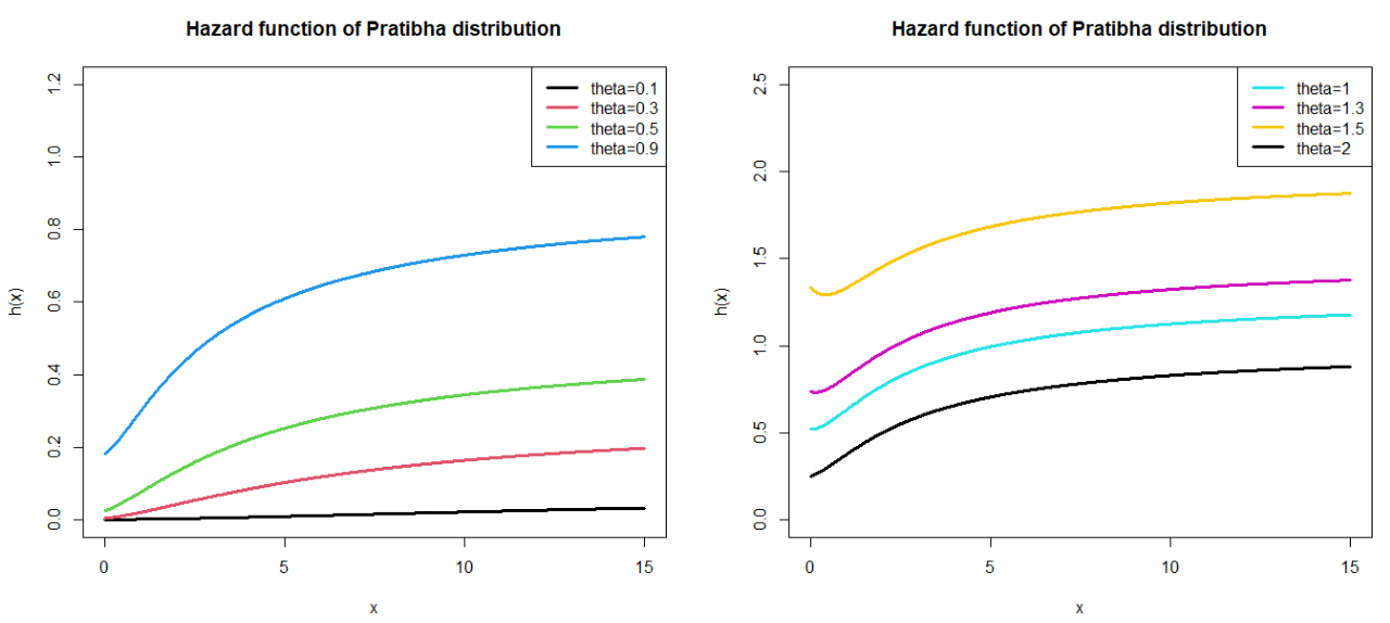
Figure 3 The hazard function of Pratibha distribution for selected values of the parameter.
Mean residual life function
Let be a random variable, defined over the support
, representing the lifetime of a component or system. Mean residual life (MRL) function measures the expected value of the remaining lifetime of the component or system, provided it has survived up to time
. Let us consider the conditional random variable
. Then, the MRL function, denoted by
, is defined as
The MRL function of Pratibha distribution can thus be obtained as
.
This gives
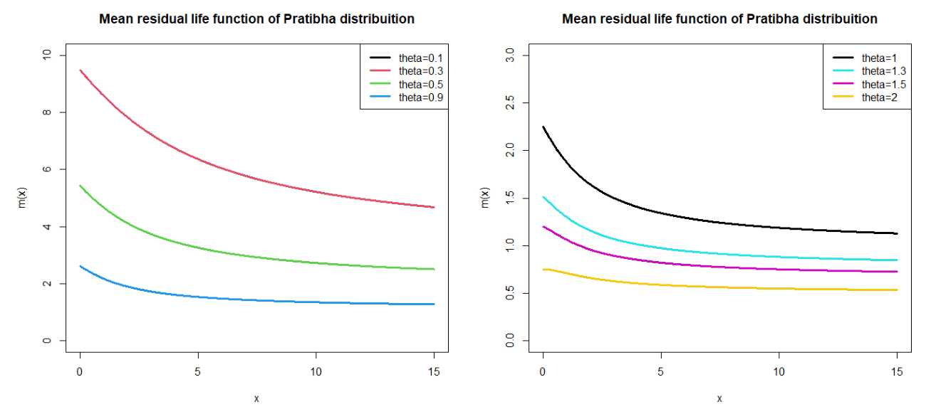
. The behaviour of the MRL of Pratibha distribution for various values of parameter
is shown in the following Figure 4. The MRL function is monotonically decreasing.

Figure 4 The mean residual life function of Pratibha distribution for selected values of the parameter.
Stochastic ordering
In Probability theory and statistics, the stochastic order quantifies the concept of one random variable being bigger than another random variable. A random variable
is said to be smaller than a random variable
in the
- Stochastic order
if
for all x
- Hazard rate order
if
for all
iii. Mean residual life order
if
for all
- Likelihood ratio order
if
decrease in
The following results due to Shaked & Shantikumar10 are well known for establishing stochastic ordering of distributions
Theorem: Let
Pratibha distribution
and
Pratibha distribution
. If
, then
hence
,
and
.
Proof: We have
We have,
Therefore,
Thus, for
,
. This means that
hence
,
and
.
Moments based descriptive measures
As we know that the moments are essential for a distribution to determine the descriptive nature of the distribution including coefficient of variation, skewness, kurtosis and index of dispersion. The
th moment about origin
of Pratibha distribution can be obtained as
Substituting
in the above equation, the first four moments about origin of Pratibha distribution can be obtained as
,
,
.
The moments about the mean, using relationship between moments about the mean and the moments about the origin, of Pratibha distribution can thus be obtained as
The descriptive measures including coefficient of variation (CV), coefficient of skewness (CS), coefficient of kurtosis (CK) and the index of dispersion (ID) of Pratibha distribution are thus obtained as
Behaviour of coefficient of variation, coefficient of skewness, coefficient of kurtosis and index of dispersion for changing values of parameter are shown in the Figure 5.
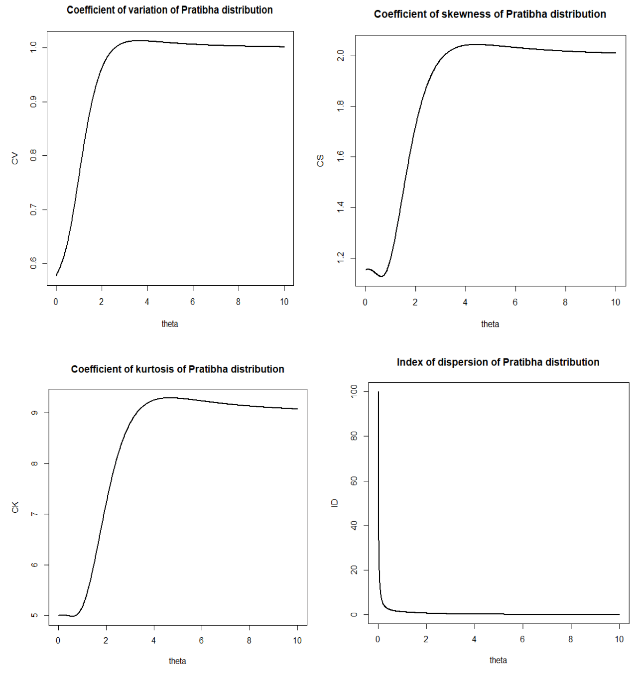
Figure 5 CV, CS, CK and ID of Pratibha distribution for different values of the parameter.
To see the comparative study of the level of over-dispersion, equi-dispersion and under-dispersion of the Pratibha, Shanker, Sujatha, Akash, Komal, Garima, Lindley, and exponential distributions for varying values of their parameter are computed and presented in the following Table 1.
|
Sl. No
|
Distributions
|
Over-dispersion
|
Equi-dispersion
|
Under- dispersion
|
|
1
|
Pratibha
|
|
|
|
|
2
|
Shanker
|
|
|
|
|
3
|
Sujatha
|
|
|
|
|
4
|
Akash
|
|
|
|
|
5
|
Komal
|
|
|
|
|
6
|
Garima
|
|
|
|
|
7
|
Lindley
|
|
|
|
|
8
|
Exponential
|
|
|
|
Table 1 Over-dispersion, equi-dispersion and under-dispersion of Pratibha, Shanker, Sujatha, Akash, Komal, Garima, Lindley, and exponential distributions for varying values of their parameter
To have a better understanding of the over-dispersion, equal-dispersion and under-dispersion of the Pratibha distribution, the behaviour of the mean and the variance of Pratibha distribution for varying values of parameter have been shown in the following Figure 6.
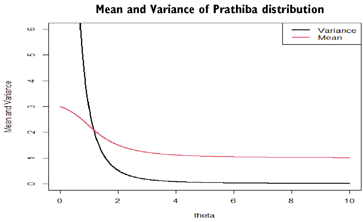
Figure 6 The nature of mean and variance of Pratibha distribution for varying values of parameter.
Deviations from mean and median
Mean deviation about the mean and the mean deviation about median of a random variable
having pdf
and cdf
are defined by
and
respectively, where
and.
Using pdf and expressions for the mean of Pratibha distribution, we get
Using above expressions some algebraic simplifications, the mean deviation about the mean
, and the mean deviation about the median
of Pratibha distribution are obtained as
Stress-strength reliability of Pratibha distribution
Let us suppose that
and
be independent strength and stress random variables having Pratibha distribution with parameter
and
, respectively. Then
is known as stress-strength parameter and is a measure of the component reliability. Thus, the stress-strength reliability of Pratibha distribution can be obtained as
Parameter estimation of Pratibha distribution
Method of moment estimate
Suppose
be a random sample of size
from Pratibha distribution with sample mean
. Equating the population mean with the corresponding sample mean, the method of moment estimate (MOME) of parameter
of Pratibha distribution is the solution of the following fourth degree polynomial equation
Maximum likelihood estimate
Suppose
be a random sample of size
from Pratibha distribution. The log likelihood function,
of Pratibha distribution is given by
The maximum likelihood estimate (MLE)
of the parameter
of Pratibha distribution is the solution of the following log likelihood equation
The above equation can easily be solved using Newton-Raphson method where the initial value of the parameter
may be taken as given by the MOME.
A simulation study
In this section, we carried out simulation study to examine the performance of maximum likelihood estimator of the Pratibha distribution. We examined the mean estimates, biases (B), mean square errors (MSEs) and variances of the maximum likelihood estimates (MLE). The mean, bias, MSE and variance are computed using the formulae
,
,
,
.
The simulation results for different parameter values of Pratibha distribution are presented in Table 2 respectively. The steps for simulation study are as follows:
- Data is generated using the acceptance-rejection method of simulation. The acceptance-rejection method is a commonly used approach in simulation studies to generate random samples from a target distribution when inverse transform method of simulation is not feasible or efficient. Acceptance- rejection method for generating random samples from the Pratibha distribution consists of following steps.
- Generate a random variable Y distributed as exp
- Generate U distributed as Uniform
- If
, then set
(“accept the sample”); otherwise (“reject the sample”) and if reject, then repeat the process step (i-iii) until getting the required samples. Here
is a positive constant.
- The sample sizes are taken as
- The parameter values are set as values
and
- Each sample size is replicated 10000 times.
The results obtained in Table 2 show that as the sample size increases, biases, MSEs and variances of the MLEs of the parameter become smaller respectively. This result is in line with the first-order asymptotic theory.
|
Parameters
|
Sample size (n)
|
Mean
|
Bias
|
MSE
|
Variance
|
| |
25
|
0.20577
|
0.00577
|
0.00024
|
0.00020
|
| |
50
|
0.20398
|
0.00398
|
0.00013
|
0.00012
|
|
|
100
|
0.20287
|
0.00287
|
0.00010
|
0.00009
|
| |
200
|
0.20189
|
0.00189
|
0.00008
|
0.00007
|
| |
300
|
0.20149
|
0.00149
|
0.00005
|
0.00005
|
| |
25
|
0.51868
|
0.01868
|
0.00076
|
0.00050
|
| |
50
|
0.51092
|
0.01092
|
0.00061
|
0.00049
|
|
|
100
|
0.51027
|
0.01027
|
0.00058
|
0.00048
|
| |
200
|
0.50925
|
0.00925
|
0.00052
|
0.00043
|
| |
300
|
0.50855
|
0.00855
|
0.00038
|
0.00031
|
Table 2 The Mean values, Biases, MSEs and Variances of Pratibha distribution for parameter values
and
An application
The application and the goodness of fit of Pratibha distribution has been discussed with one real life example. As we have seen that Pratibha distribution is highly positively skewed, so following positively skewed dataset has been considered.
Dataset-1: The following right skewed complete data discussed in Murthy et al.11 regarding the failure times of 24 mechanical components are considered and the observations are:
30.94, 18.51, 16.62, 51.56, 22.85, 22.38, 19.08, 49.56, 17.12, 10.67, 25.43, 10.24, 27.47,
14.70, 14.10, 29.93, 27.98, 36.02, 19.40, 14.97, 22.57, 12.26, 18.14, 18.84.
|
Min
|
1st Quartile
|
Median
|
Mean
|
3rd Quartile
|
Max
|
|
10
|
16.21
|
19.24
|
22.97
|
27.6
|
51.56
|
The descriptive Summary of the dataset -1 is as follows:
The goodness of fit of the distributions is based on the values of
, AIC (Akaike Information Criterion) and K-S (Kolmogorov-Smirnov) statistic. AIC and K-S are computed using
,
, where
= the number of parameters,
= the sample size and
is the empirical distribution function. The distribution having lower
, AIC, and K-S are said to be best distribution. The MLE
and standard error, S.E
of
,
, AIC, K-S and p-value of the fitted distributions are presented in the Table 3.
It is obvious from the goodness of fit in the Table 3 that the Pratibha distribution provides much closer fit than exponential, Lindley, Garima, Komal, Akash, Sujatha and Shanker distributions. Therefore, the Pratibha distribution can be considered as an important lifetime distribution for modeling positively skewed lifetime data from biomedical sciences and engineering.
|
Sl. No
|
Distributions
|
MLE
and SE
|
|
AIC
|
K-S
|
p-value
|
|
1
|
Pratibha
|
0.1278 (0.0150)
|
178.82
|
180.82
|
0.14
|
0.71
|
|
2
|
Shanker
|
0.0866 (0.0124)
|
184.39
|
186.39
|
0.23
|
0.17
|
|
3
|
Sujatha
|
0.1273 (0.0149)
|
179.02
|
181.02
|
0.16
|
0.54
|
|
4
|
Akash
|
0.1298 (0.0152)
|
178.45
|
180.45
|
0.15
|
0.61
|
|
5
|
Komal
|
0.1000 (0.0144)
|
187.57
|
189.57
|
0.35
|
0
|
|
6
|
Garima
|
0.1000 (0.0168)
|
199.68
|
201.68
|
0.23
|
0.15
|
|
7
|
Lindley
|
0.0837 (0.0121)
|
185.76
|
187.76
|
0.30
|
0.03
|
|
8
|
Exponential
|
0.0435 (0.0088)
|
198.44
|
200.44
|
0.33
|
0.02
|
Table 3 ML estimate with their standard error,
, AIC, K-S and p-value of the considered distributions for the data set-1
Concluding remarks and future works
In this paper an attempt has been made to propose a new one parameter lifetime distribution named Pratibha distribution. Statistical properties, estimation of parameter and application of the distribution has been discussed and presented. As the distribution is new one, it is expected and hoped that it will be of great use to statisticians working in the field of data science to model lifetime data from different fields of knowledge. Being a new lifetime distribution with flexibility, tractability and practicability, a lot of future works can be done on Pratibha distribution.
Conflicts of interest
The author declared that there is no conflicts of interest.
Acknowledgments
Author is grateful to the editor-in-chief and the anonymous reviewer for quick and constructive comments which improved the quality of the paper.
Funding
References
- Lindley DV. Fiducial distributions and Bayes’ theorem. Journal of the Royal Statistical Society, Series B. 1958;20(1):102–107.
- Shanker R. Shanker distribution and its applications. International Journal of Statistics and Applications. 2015a;5(6):338–348.
- Shanker R. Akash distribution and its applications. International Journal of Probability and Statistics. 2015b;4(3):65–75.
- Shanker R. Sujatha distribution and its applications. Statistics in Transition-New Series. 2016a;17(3):391–410.
- Shanker R. Garima distribution and Its application to model behavioral science data. Biom Biostat Int J. 2016b;4(7):275–281.
- Shanker R. Komal Distribution with properties and Application in Survival Analysis, Biometrics & Biostatistics International Journal. 2023;12(2):40–44.
- Shanker R, Hagos F, Sujatha S. On modeling of lifetimes data using exponential and Lindley distributions. Biom Biostat Int J. 2015;2(5):140–147.
- Shanker R, Hagos F, Sujatha, S. On modeling of lifetime data using one parameter Akash, Lindley and exponential distributions. Biom Biostat Int J. 2016;3(2):54–62.
- Shanker R, Hagos F. On modeling of lifetime data using Akash, Shanker, Lindley and exponential distributions. Biom Biostat Int J. 2016;3(6):214–224.
- Shaked M, Shanthikumar JG. Stochastic orders and their applications. New York: Academic Press; 1994.
- Murthy DNP, Xie M, Jiang R. Weibull models. New York: John Wiley & Sons; 2004.

©2023 Shanker. This is an open access article distributed under the terms of the,
which
permits unrestricted use, distribution, and build upon your work non-commercially.


