The study of Micronutrients in Ntanwaogba Creek were thoroughly carried out to monitor its rates of deposition at different numerous discharge location sites in the study environment, this was imperative because the rates of biological waste discharge at regular interval, based on this factor, it was necessary to conduct a comprehensive investigation of their rate of concentration at different station point of discharge. This implies that the rate of dispersions from the contaminant influenced constant discharge of waste in the creek, and based on these factors, it was determined that such comprehensive research was required. Micronutrients act as a substrate for microbial growth, but the speed at which they are injected into the rill affects how quickly they move through the system. In order to determine the effects of these two parameters on the migration rate of faecal coliform at different point sources of discharge, the study observed different growth rate at different station point in the study location. This observed condition indicates that the pollutants had a range of development speeds, including both slow and fast, which was enabled by these considerations. The system discovered that lower velocities have an effect on velocity rates with higher concentrations, and that accumulation with micronutrients increased their concentration. However, the concentration rates varied depending on the dominant characteristics of the transport under pressure at various points of discharge. In the simulation, these two parameters were used to determine the various pressure rates at different station points. Unquestionably, the study has depicted the effects of these two parameters' pressures on the movement of faecal coliform in a range of figures that correspond to the several point sources of discharge looked at. The speeds recorded at various station locations represented the pressure rates at various rates of concentration in the research environment. It has established the scope of the influence of rill flow velocity and the variance in micronutrient deposition at various point sources. On the basis of model simulation prediction results, also, the dispersions at various point sources were evaluated. Both parameters showed correlations for the best fits when the predicted and experimental values were compared for model validation.

Keywords: modeling, transport, fecal coliform, micronutrients and dispersion coefficient

Many studies have shown that water-borne infections are extremely dangerous to human health. These facts make it clear that, if pollution rates are not controlled, there will always be significant hazards to the overall health of the ecosystem. Total Maximum Daily Load (TMDL) implementation costs were assessed by experts, and they range from $0.9 to $4.3 billion annually.^1,2 The main factor causing stream impairments is pathogen influxes from land-based agricultural activities.^2,3 Controlling pathogen contamination caused by cattle, meantime, is a difficult task. Riparian buffers can be fenced off to prevent pathogen contamination; however it is not apparent how broad the buffers need to be to be effective in preventing pathogen contamination of stream water.⁴ The research that has thoroughly evaluated studies in this field has elaborated on the pathogen contamination of stream water ^4–8 (Jamieson. More research has concentrated on understanding pathogen transmission in stream water using mathematical models.^5,6,9,10 Also, the principal source of drinking water is typically a surface reservoir, indicating that these bodies of surface water are frequently subjected to pathogen pollution.^9,11–13 There has been a considerable improvement in knowledge of water quality and water treatment for pathogen pollution in industrialized nations because specialists tracked the occurrences of 26 water-borne illnesses through public water sources, which were done by experts.^12–21 Also, the inflow of contaminated stream water into lakes and reservoirs during the rainy seasons might result in a significant rise in pathogen rates.^4,22–24 For purposes of measuring the quantity of pathogen uptake from torrents running into lakes and reservoirs during wet seasons it also involved monitoring pathogen movement including its dispersion.^2,3,25

$\frac{dc}{dx}+\beta (x) K=A(x)$   1

Nomenclatures

C = Concentration

B = Micronutrients

K = Dispersions. Velocity of flow

A= Fluid Density

X = Distance

Multiplying the equation through by $C[x]$ , we have:

$C(x) \frac{dC}{dx}+C(x) \beta (x) K=C(x) A(x)$   2

Let $P(x)=C(x) \beta (x)$   3

Then Equation (2), we have:

$C(x) \frac{dC}{dx}+C(x) \beta (x) K=C(x) A(x)$   4

$C(x) \frac{dC}{dx} + P(x) K=C(x) A(x)$   5

$C(x) P^1+ P(x) K= C(x) A\left(x\right)$   6

$C(x) P^1=C(x) A-P(x) K$   7

Differentiate 2^nd term on the left hand side of (6) with respect to x, we have

$K \frac{dC}{dx}= C\left(x\right)A\left(x\right)- C\left(x\right) P^1$   8

$\frac{dC}{dx}= \frac{1}{K}\left[ C\left(x\right)A\left(x\right)-C\left(x\right)P^1 \right]$   9

$\frac{dC}{dx}= \frac{C\left(x\right)}{K} \left[A\left(x\right)-P^1\right]$   10

Applying separation of variables, by dividing through by C(x) and cross multiply by dx, gives:

$\frac{dC}{C}=\frac{1}{K} \left[A\left(x\right)-P^1\right] dx$   11

$\frac{1}{C\left(x\right)} dC=\frac{1}{K} \left[A\left(x\right)-P^1\right] dx$   12

$\frac{1}{C\left(x\right)} dC= \left(\frac{A\left(x\right)}{K}-\frac{P^1}{K}\right) dx$   13

${\displaystyle \int \frac{1}{C\left(x\right)}} dC={\displaystyle \int \left( \frac{A\left(x\right)}{K}- \frac{P^1}{K} \right)} dx+\eta$   14

$\ln C\left(x\right)={\displaystyle \int A\left(x\right) }dx-{\displaystyle \int \frac{P^1}{K}} dx+\eta$   15

$\ln C\left(x\right)= \frac{1}{K} \left[Ax-P^1\right] x+\eta$   16

$\ln C\left(x\right)=\left(\frac{A(x)}{K}- \frac{P^1}{K}\right) x+\eta$   17

Taking exponent of the both side of the equation

$C\left(x\right)=\ell { }^{\left( \frac{A\left(x\right)}{K} - \frac{P^1}{K} + \eta \right)}$   18

$C\left(x\right)=D\ell { }^{\frac{1}{K} }{}^{\left( Ax- P^{1}x \right)}$   19

The water samples were taken sequentially according to the requirements set forth at various places. These samples were obtained at various locations, which resulted in fluctuations at various distances, resulting in variable faecal coliform concentrations, and the experimental results were compared. Using the conventional procedure for the experiment at several samples at various stations, a typical laboratory experiment was carried out to track faecal coliform.

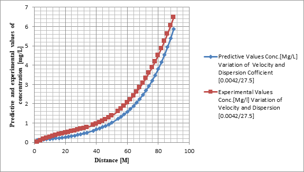
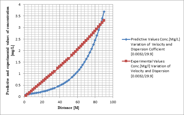
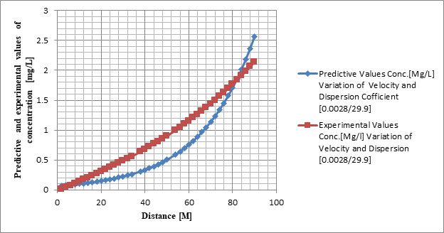
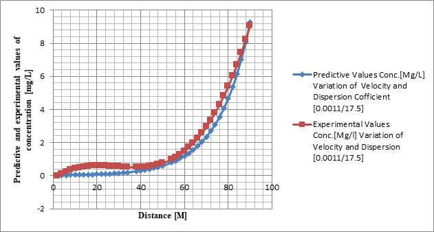
(Table 1-6)(Figure 1-6) shows how the major influencing factors in the research environment affect the migration rate of faecal coliform. The variance of the contaminant's exponential growth rate in terms of quick and slow growth in relation to increase in distance was depicted in the figures. However, during the transport system's exponential phase. The observed fluctuations are primarily related to the pace of micronutrient depositions, including dispersion from the pollutant at several station locations, where the starting concentrations are recorded. The growth rate's behaviour did exhibit some degree of variability. Such a condition shows that the concentration change rate at different study locations was determined by the micronutrient's function as a substrate for any bacterium. The study looked at these pressures from transport and the impact that condition had on the flow dynamics that pushed the microorganisms at different station points of discharge. The many types of micronutrient depositions that have been seen in the rill and the fluctuations in those depositions as a whole have affected the growth rate of faecal coliform in the study region, as shown in graphical representation in all of the figures. The behaviour of faecal coliforms was monitored through the use of modeling and simulation by examining the variable effect of contaminant movement at distinct station points of discharge. The experimental and prediction values of each created figure expressed best fit correlations.

Figure 1 Model Prediction and Experimental Values on Fecal Coliform Concentration at Various Distances.

Figure 2 Model Prediction and Experimental Values on Fecal Coliform Concentration at Various Distances.

Figure 3 Shows the model's Prediction and Experimental Values for Faecal Coliform Concentrations at Various Distances.

Figure 4 Shows the model's Prediction and Experimental Values for Faecal Coliform Concentrations at Various Distances.

Figure 5 Model Prediction and Experimental Values on Fecal Coliform Concentration at Various Distances.

Figure 6 Model Prediction and Experimental Values on Fecal Coliform Concentration at Various Distances.

The system keeps track of the contaminant's behaviour at several station points of discharge that are seen in the research environment. An experimental approach was used to monitor the station points, and it led to concentration variations at various stations spaced uniformly apart. The microorganisms' growth-related behaviour was evaluated, thus, it was found that the concentration of faecal coliform in Ntanwaogba Creek increased gradually and quickly. To identify the variables influencing the faecal coliform's transport behaviour, the reaction of the organism in the rill was evaluated. The pollutant was observed to rise at various station sites in response to micronutrients identified in various stations that support the behaviour, demonstrating the contrast between their effects on the concentration's slow and fast stages of growth.

None.

None.

The authors declare that they have no competing interests.

1. U.S. Environmental Protection Agency. WATERS (Watershed Assessment, Tracking & Environmental ResultS). Washington, D.C. 2010a.
2. US Environmental Protection Agency (US EPA). Impaired waters and total maximum daily loads. 2012.
3. Pandey PK. Modeling in- stream Escherichia coli concentrations. Graduate Dissertation Iowa state university. 2012:62–75.
4. Nagels JW, Davies-Colley RJ, Donnison AM, et al. Faecal contamination over flood events in a pastoral agricultural stream in New Zealand. Water Sci Technol. 2002;45(12):45–52.
5. Pachepsky YA, Sadeghi AM, Bradford SA, et al. Transport and fate of manure-borne pathogens: Modeling perspective. Agricultural Water Management. 2006;86(1–2):81–92.
6. Jamieson R, Gordon R, Joy D, et al. Assessing microbial pollution of rural surface waters: A review of current watershed scale modeling approaches. Agricultural Water Management. 2004;70(1):1–17.
7. Jamieson R, Joy DM, Lee H, et al. Transport and deposition of sediment-associated Escherichia coli in natural streams. Water Res. 2005;39(12):2665–2675.
8. Jamieson RC, Joy DM, Lee H, et al. Resuspension of sediment-associated Escherichia coli in a natural stream. J Environ Qual. 2005;34(2):581–589.
9. Kim JW, Pachepsky YA, Shelton DR, et al. Effect of streambed bacteria release on E. coli concentrations: Monitoring and modeling with the modified SWAT. Ecological Modeling. 2010;221(12):1592–1604.
10. Muirhead RW, Davies-Colley RJ, Donnison AM, et al. Faecal bacteria yields in artificial flood events: quantifying in-stream stores. Water Res. 2004;38(5):1215–1224.
11. Eluozo SN, Amadi CP. Velocity and Oxygen Deficit Influence on the Transport of Francisela in Eleme Creek. Journal of Water Resource Engineering and Management. 2019;6(2):43–48.
12. Eluozo SN, Afiibor BB. Mathematical model to monitor the transport of bordetella influenced by heterogeneous porosity in homogeneous gravel depositions. Journal of Geotechnical Engineering. 2019;6(1).
13. Ezeilo FE, Eluozo SN. Linear Phase Velocity Effect on Accumulation of Zinc in Homogeneous Fine Sand Applying Predictive Model. International Journal of Mechanical and Civil Engineering. 2018;4(4):17–32.
14. Eluozo SN, Ezeilo FE. Numerical Modeling of Nocardia Migration Influenced Transport Pressured by Dispersion and Velocity in Fine Sand Formation in Wetland Environment. Journal of Water Resources Engineering and Management. 2018;5(1):25–32.
15. Eluozo SN, Ezeilo FE. Modeling Heterogeneous Porosity in Alluvia Plain Deposition in Deltaic Formation. Recent Trend in Civil Engineering & Technology. 2018;8(2):1–10.
16. Ezeilo FE, Eluozo SN. Dispersion and storage coefficient influences on accumulation of frankia transport in heterogeneous silty and fine sand formation, Warri, Delta State of Nigeria. International Journal of Mechanical and Civil Engineering. 2018;4(4):1–16.
17. Eluozo SN, Amadi CP. Modeling and simulation of legionella transport influenced by heterogeneous velocity in stream. Journal of Water Resource Engineering and Management. 2019;6(2):25–31.
18. Eluozo SN, Ezeilo FE. Predicting the behaviour of borrelia in homogeneous fine sand in coastal area of Bakana. Recent Trend in Civil Engineering & Technology. 2018;8(2):1–19.
19. Eluozo SN, Oba AL. Modeling and simulation of cadmium transport influenced by high degree of saturation and porosity on homogeneous coarse depositions MOJ Civil Engineering. 2018;4(4):263–267.
20. Eluozo SN, Afiibor BB. Dispersion and dynamics influences from phosphorus deposition on e-coli transport in coastal deltaic Lake. MOJ Applied Bionics and biomechanics. 2018;2(5):289–293.
21. Eluozo SN, Oba AL. Predicting heterogeneous permeability coefficient pressured by heterogeneous seepage on coarse deposition. MOJ Civil Engineering. 2018;4(4):257–261.
22. Brookes JD, Antenucci J, Hipsey M, et al. Fate and transport of pathogens in lakes and reservoirs. Environment International. 2004;30(5):741–759.
23. Howe AD, Forster S, Morton S, et al. Cryptosporidium oocysts in a water supply associated with a cryptosporidiosis outbreak. Emerg Infect Dis. 2002;8(6):619–624.
24. Gibson CJ, Haas CN, Rose JB. Risk assessment of waterborne protozoa: current status and future trends. Parasitology. 1998;117:S205–S212
25. Kistemann T, Classen T, Koch C, et al. Microbial load of drinking water reservoir tributaries during extreme rainfall and runoff. Applied and Environmental Microbiology. 2002;68(5):2188–2197.