The design of the four legged walking robot “PASIQUAD” is presented in this article. It was designed in the university Carlos III of Madrid. It is a quadruped quasi–passive robot (with only one motor/actuator). The manuscript is focused on how the PASIQUAD walks and the kinematics and dynamics of the movement. In the manuscript the position, velocity and acceleration of each of its parts, as well as all the forces and torques on each of them, motor torque included, will be explain. The PASIQUAD robot copy the movement of animals and it is almost passive. That is a big advantage in energy cost.

Keywords: robotics, passive, walking robots, quadruped, design

Nowadays, walking robots is one of the main research priority areas. However mobile robots are not adapted to be used in domestic environments, due to their large volume and/or weight, and their lack of maneuverability in these complex scenarios. Currently, the interest in the development of robots is increasing and it is being investigated by a great number of research groups in the entire world.^1,2 The development of robots that copy movements from animals, like bipedal walking or quadruped, is of major interest in robotics.³ As a result, a wide variety of refined designs have been proposed.⁴ Pfeifer R & Bongard J^5–7 explains how the new robotics employs ideas and principles from biology (biomechanical studies). Normally, walking robots are designed by a high number of actuators, that are used for controlling the high degrees of freedom (DOF).^8,9 On the other hand, one of the major drawbacks in robots is the power consumption and the weight. In the majority of them, around 30% of the total weight is due to the actuators and wires, and more than 25% is due to the reduction systems coupled.¹ For this reason, our work is focused on the design of new mechanisms and kinematic chains which, maintaining the robot capabilities, require smaller number of actuators. This would reduce the robot mass and hence, its power consumption and total cost. The introduction of new mechanisms and kinematic chains enables walking robot designs with fewer actuators and gearboxes, thereby reducing the weight, power consumption and cost of operation without compromising walking functionality.

Different research groups have developed robots based on passive walking techniques in the last years¹⁰: Robot Ranger of Cornell University,¹¹ Robot Toddlers from MIT University,¹² Robot Denise from Delft University,¹³ the quadruped Puppy developed by Iida F¹⁴ and the last robot of interest in the passive theory is the one developed in the Nagoya Institute of Technology.^15,16 Most of the proposed solutions are based on human or animal legs, where the links are connected by joints (hip, knee and ankle), all or most of which are operated by actuators (such as motors, pneumatic devices and artificial muscles).¹⁷ Alternatively, researchers aim to emulate the walking motion by combining various classical mechanisms. Ceccarelli and his team, working from the latter perspective, at the Laboratory of Robotics and Mechatronic (LARM) have presented the biped robot EP–WaR II.¹⁸ More recently, the group has developed low–cost humanoid legs Caluma¹⁹ and has begun working on other designs. The MAQLAB group of the Universidad Carlos III de Madrid, from the same perspective, has designed and manufactured one walking biped.^20,21 In this article, we present a walking robot, called PASIQUAD, with low DOF, which represents a qualitative improvement in the service robotic field service. The innovative design has been carried out with the combination of classical mechanisms.²² The proposed mechanism is an arrangement of links in planar movement that has only one DOF In this manuscript, the planar kinematics and dynamics analysis of PASIQUAD is presented. The study is performed from a theoretical point of view, and aims to obtain the linear and angular position coordinates, velocities and accelerations for all links, as well as all the forces and torques between links including motor torque, for any time in the course of one step. The biped PASIQUAD mechanism, defining its subassemblies and parts, as well as the nomenclature used is descript in the section “PASIQUAD”; next, how to deduce the expressions for the angular and linear position, velocities and accelerations for all the links of the walking robot is explained in the section “Kinematics of “PASIQUAD”; then, the method to obtain all the forces and torques on every link, at every time in the course of one step of PASIQUAD is exposed in the “Dynamics of PASIQUAD”; and at the last section, the conclusions of this work are presented.

In order to descript the quadruped presented in this article (Figures 1–4), it be divided into two essential mechanisms:

1. The Chebyshov mechanism (Quasi–straight line generator)
2. The pantograph (Amplifier mechanism)

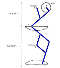
Figure 1 Chebyshov-Pantograph mechanism and the trajectories of interest.

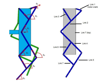
Figure 2 Angular positions for the links.

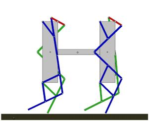
Figure 3 PASIQUAD while is walking.

Figure 4 A track for a PASIQUAD (from J1= p/2 to 5p/2 rad).

The coupling Chebyshov–pantograph mechanism and trajectories tracked are shown in Figure 1. The Chebyshov mechanism transfers the rotational movement of the motor into a continuous cyclical trajectory, which is formed by a quasi–straight section and a curved one, point C in Figure 1. As is show in Figure 1 this mechanism is then linked to a pantograph mechanism which moves and inverts the trajectory of the point C in the point E. Note than the point D is fixed. The ratio of magnification of the pantograph is one in the PASIQUAD, however, it could be modified to amplify or decrease. Thanks of this leg the movement are forced. The two front legs are phased out just the opposite of the back legs to obtain the stability in every moments of the step. While the right front leg and the left back leg are flying the left front leg and the right back leg are in the floor, and so on. The points A, B and D (Figure 1) are fixed at the link T called “hip”. The opposite leg is phased out p rad and connected to the same motor crack, link 1. In Figure 3 the supporting legs and flying legs are shown in green and blue and the link 1 in red (Figure 2). Angular positions for the links; nomenclature and numeration for the supporting leg, the members of the opposite leg will be named with primes. As can be seen in Figure 2, each link of the flying leg (green one) has been numerated and named, using prime (x’), to distinguish from those belonging to the supporting leg (blue one). Each leg has 7 links, but since the motor crank (link number 1) is shared with both legs (hence, there is no link number 1’), the number of links for PASIQUAD, including the single hip (link T) is 14. The Figure 4 shows a sequence for one step of PASIQUAD. It was simulated with a mechanical program (Working Model 2D). Note that the right and left legs are opposite in front and back.

The kinematical study is focused only on the front (two front legs and front hip), the back is the same with the right and left switched values. The kinematical study presented here is related to one PASIQUAD’s step, having one of its feet (the supporting foot) always in contact with a horizontal surface (x axis). No relative motion between the supporting foot and the ground is considered, so this foot could be referred to as the ground element. Taking into account this, the PASIQUAD is a planar mechanism with one DOF, so the angular positions of any link can be obtains in function of the angular position of the motor crank (θ1):

$\theta i=\theta i\left(\theta 1\right),i=1,2,,\mathrm{...1}\text{'},2\text{'}\mathrm{...}$ (1)

Knowing the angular positions of any link in function of the angular position of the motor crank (θ 1), the centers of mass of every links can be expressed in function of the angel of the motor crank (θ 1).

$xi=xi\left(\theta 1\right);yi=yi\left(\theta 1\right),i=1,2,,\mathrm{...1}\text{'},2\text{'}\mathrm{...}$ (2)

The angular position of the motor crank (θ1) is a time dependent function, then the positions of every link and their angels are also a knowing time dependent functions. The linear velocities and accelerations of the center of mass and the angular velocity and accelerations of every link are calculated by taking the first and second derivatives of the functions of the positions and the angles mentioned above. Actually, the robot kinematics is based on two close loop kinematic chains (one for each mechanism previously described) which lead to the following two equations systems (The dimensions of the links have been particularized for the designed PASIQUAD, so that l1=1):

The chain of chebyshov mechanism (links number 1, 2, 3 and T)

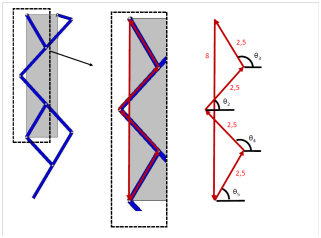
In a Chebyshov mechanism, the distance between link 1, motor crank, and fixed crank, link 3, (a and b in Figure 1, respectively) is 2l1, the length of the link 3 is 2.5l1, the length of link 2 is 5l1, and the link 3 and link 2 are joined at the middle point of the latter. The close loop of the kinematic chain of Chebyshov mechanism is (Figure 5):

$-2.5e^{j{\vartheta }_2}+2.5e^{j{\vartheta }_3}+e^{j{\vartheta }_1}+2=0$ (3)

The projection equations are written in a Euler’s formula. See Eqs. (3) to (5), where were j is the imaginary unit.

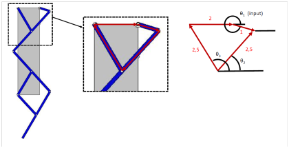
Figure 5 The chain of Chebyshov mechanism .

The chain of pantograph mechanism (links number 2, 3, 4, 6 and T)

In our model, the distance between fixed point B and D is 8l1, so the close loop of the kinematic chain of the pantograph is (Figure 6):

$2.5e^{j{\vartheta }_2}+2.5e^{j{\vartheta }_3}+2.5e^{j{\vartheta }_4}+2.5e^{j{\vartheta }_5}-8j=0$ (4)

Figure 6 Pantograph chain.

The x–projection and y–projection of the two close loops are shown below:

$\{\begin{array}{l}-2.5\cdot \cos ({\theta }_2)+2.5\cdot \cos ({\theta }_3)+\cos ({\theta }_1)+2=0\\ -2.5\cdot \sin ({\theta }_2)+2.5\cdot \sin ({\theta }_3)+\sin ({\theta }_1)=0\end{array}$

$\{\begin{array}{l}\cos ({\theta }_4)+\cos ({\theta }_5)+\cos ({\theta }_2)+\cos ({\theta }_3)=0\\ \sin ({\theta }_4)+\sin ({\theta }_5)-3.2+\sin ({\theta }_2)+\sin ({\theta }_3)=0\end{array}$ (5)

Solving the system of equations of the close loop of the Chevyshov:

$\{\begin{array}{l}{q}_2=acos(\frac{-4\times cos{(q_1)}^2-13\times cos(q_1)-10+sin(q_1)\times \sqrt{(-16\times {(cos(q_1))}^2+60\times cos(q_1)+100)}}{-25-20\times cos(q_1)})\\ q_3=acos(\frac{-4\times cos{(q_1)}^2-13\times cos(q_1)-10-sin(q_1)\times \sqrt{-16\times cos{(q_1)}^2+60\times cos(q_1)+100})}{25+20\times cos(q_1)})\end{array}$ (6)

And, the solution of the close loop of the Pantograph: expression for the second system (in function of the first systems solutions)

$\{\begin{array}{l}{\theta }_4=a\cos (\frac{(\cos ({\theta }_2)+\cos ({\theta }_3))\cdot (-(D^2+C^2))+((sin({\theta }_2)+\sin ({\theta }_3)-3.2)\cdot \sqrt{(4\cdot (D^2+C^2)-{(-(D^2+C^2))}^2)}}{2\cdot (D^2+C^2)})\\ {\theta }_5=a\cos (\frac{(\cos ({\theta }_2)+\cos ({\theta }_3))\cdot (-(D^2+C^2))-((sin({\theta }_2)+\sin ({\theta }_3)-3.2)\cdot \sqrt{(4\cdot (D^2+C^2)-{(-(D^2+C^2))}^2)}}{2\cdot (D^2+C^2)})\end{array}$ (7)

Where ${\mathrm{D}}^2+C^2=12.24-6.4sin(q_2)-6.4sin(q_3)+2sin(q_2)sin(q_3)+2cos(q_2)cos(q_3)$

Note that the solution of the close loop of the Pantograph is in function of the Chebyshov system solutions. These equations determine the angles for all the links as functions of the angle of the motor crank, θ1, which is also a function of time. The others values of angles involved are the same to one of the given ones in the Eqs. (6) to (8), in particular (Figure 2):

$\begin{array}{l}{\vartheta }_6={\vartheta }_5\\ {\vartheta }_7={\vartheta }_4\end{array}$ (8)

A phase out of p radians on J₁ is applied for the links belonging to the opposite leg:

${\vartheta }_i\left({\vartheta }_1\right)={\vartheta }_i\left({\vartheta }_i+\pi \right)$ (9)

The positions of the center of mass for all the links are easily obtained using trigonometric relations (for example, x5=L5cosJ₅/2, y5=L5sinJ₅/2; x4=L5cosJ₅+L4cosJ₄/2, y4=L5sinJ₅+L4sinJ₄/2; and so on). Then, the linear velocity and acceleration of its center of mass are calculated by time differentiating once and twice for every link. The angular velocity and acceleration for every link is founded also by time differentiating once and twice. Therefore, the kinematics of PASIQUAD for every link is solved during the whole step.

As the kinematics study, the dynamical study is focused only on the front (two front legs and front hip), the back is the same with the right and left switched values, and the overturned torque transmitted by the hip will be the opposite. The inverse dynamics, which calculates the forces and torques that produce kinematics (movement). Then inputs for the dynamical problem are the kinematic outputs. The dynamical unknowns involved are the motor torque, T, and all the forces between links, fji (exerted by link j on link i) and the torque to one hip to the other. Forces and torques acting on an i–link are shown in Figure 7.

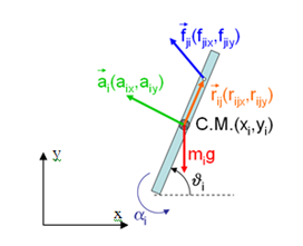
Figure 7 Forces and torques acting on a i-link.

The dynamics of i–link is described as follows where Newton’s third law has been used to reduce the number of unknown forces:

$\begin{array}{c}{\displaystyle \sum }_i{\overrightarrow{F}}_i=m_i{\overrightarrow{a}}_i\\ {\overrightarrow{f}}_{ij}=-{\overrightarrow{f}}_{ji}\\ {\displaystyle \sum }_i{T}_{oni}=I_i\alpha \end{array}\}\Rightarrow$

$\Rightarrow \{\begin{array}{l}{\displaystyle \sum }_{j<i}{f}_{j{i}_x}-{\displaystyle \sum }_{k>i}{f}_{i{k}_x}=m_i{a}_{i_x}\\ {\displaystyle \sum }_{j<i}{f}_{j{i}_y}-{\displaystyle \sum }_{k>i}{f}_{i{k}_y}=m_{i}g+m_i{a}_{i_y}\\ T_i+{\displaystyle \sum }_{j<i}\left(r_{i{j}_x}{f}_{j{i}_y}-r_{i{j}_y}{f}_{j{i}_x}\right)-{\displaystyle \sum }_{k>i}\left(r_{i{k}_x}{f}_{i{k}_y}-r_{i{k}_y}{f}_{i{k}_x}\right)=I_i{\alpha }_i\end{array}$

$i=2,3,,\mathrm{...7},T,1\text{'},2\text{'}$ (13)

Because there are 3 equations for each link, and there are 14 links, the dynamics system of the PASIQUAD consists of 42 linear equations. The linear equation system (Eq. 13) is expressed in a matrix form (Eq. 14) as follows:

 [A(42x42)]x[F(42x1)]=[I(42x1)] where

$\text{[A]=}\left[\begin{array}{ccccccccc}{\text{a}}_{\text{1,1}}& {\text{a}}_{\text{1,2}}& {\text{a}}_{\text{1,3}}& \text{.}& \text{.}& \text{.}& \text{.}& \text{.}& {\text{a}}_{\text{1,42}}\\ {\text{a}}_{\text{2,1}}& {\text{a}}_{\text{2,2}}& {\text{a}}_{\text{2,3}}& \text{.}& \text{.}& \text{.}& \text{.}& \text{.}& \text{.}\\ \text{.}& \text{.}& \text{.}& \text{.}& \text{.}& \text{.}& \text{.}& \text{.}& \text{.}\\ \text{.}& \text{.}& \text{.}& \text{.}& \text{.}& \text{.}& \text{.}& \text{.}& \text{.}\\ \text{.}& \text{.}& \text{.}& \text{.}& \text{.}& \text{.}& \text{.}& \text{.}& \text{.}\\ \text{.}& \text{.}& \text{.}& \text{.}& \text{.}& \text{.}& \text{.}& \text{.}& \text{.}\\ \text{.}& \text{.}& \text{.}& \text{.}& \text{.}& \text{.}& \text{.}& {\text{a}}_{\text{40,41}}& {\text{a}}_{\text{40,42}}\\ \text{.}& \text{.}& \text{.}& \text{.}& \text{.}& \text{.}& {\text{a}}_{\text{41,40}}& {\text{a}}_{\text{41,41}}& {\text{a}}_{\text{41,42}}\\ {\text{a}}_{\text{42,1}}& \text{.}& \text{.}& \text{.}& \text{.}& \text{.}& {\text{a}}_{\text{42,40}}& {\text{a}}_{\text{42,41}}& {\text{a}}_{\text{73,42}}\end{array}\right]$

$a_{1,1},a_{1,2},a_{1,3}\mathrm{....}{a}_{1,73},a_{2,1}\mathrm{....}{a}_{73,73}$ are the coefficients that multiply the forces.

[F] Is the vector of forces and torques. The 42 unknowns. [I] is the vector of inertias.

$\begin{array}{c}\left[\begin{array}{cccc}{a}_{11}& a_{12}& \dots & \\ a{}_{21}& a_{22}& \dots & \\ ⋮& ⋮& \ddots & ⋮\\ & & \dots & \end{array}\right]·\left[\begin{array}{c}{f}_{{12}_x}\\ f_{{12}_y}\\ ⋮\\ T_8\\ ⋮\\ {}_{}\end{array}\right]=\left[\begin{array}{c}{m}_2{a}_{2_x}\\ m_{2}g+m_2{a}_{2_y}\\ I_2{\alpha }_2\\ ⋮\\ \end{array}\right]\\ \left[A(coefficient)\right]·\left[F(force)\right]=\left[I(inertia)\right]\\ \Downarrow \\ \left[F\right]={\left[A\right]}^{-1}·\left[I\right]\end{array}$ (14)

Then, this system of equation for every position is solved via matrix inversion.

The design of a quadruped quasi–passive walking robot called PASIQUAD has been presented in this article. Also a methodology to obtain the dynamics has been presented. All the kinematics and dynamics have been solved for this robot during the walking. The main advantage is that the program is parametric, and we can modify all parameters to optimize or improve the design. In Figure 8 the complete design of PASIQUAD is shown.

Figure 8 The PASIQUAD.

None.

Author declares that there are none of the conflicts.

References

1. Hirose M, Ogawa K. Honda humanoid robots development. Philos Trans A Math Phys Eng Sci. 2007;365(1850):11–19.
2. Akachi K, Kaneko K, Kanehira N. Development of humanoid robot HRP–3P. Proceeding 5th IEEE–RAS International Conference on Humanoid Robots. 2005. p. 50–55.
3. Hasaneini SJ, Macnab CJB, Bertram, et al. The dynamic optimization approachto locomotion dynamics: human–like gaits from a minimally constrained biped model. Advanced Robotics. 2013;27(11):845–859.
4. Azimi M, Yazdi MRH. Energy dissipation rate control and parallel equations solving method for planar spined quadruped bouncing robot. J Mech Sci Tech. 2017;31(2):875–884.
5. Pfeifer R, Iida F, Bongard J. New Robotics: Design Principles for Intelligent Systems. Artificial Life. 2005;11(1–2):99–120.
6. Pfeifer R, Gomez G. Interacting with the real world: design principles for intelligent systems. Artificial life and Robotics. 2005;9(1):1–6.
7. Pfeifer R, Bongard J. How the Body Shapes the Way We Think: A New View of Intelligence. MIT Press Cambridge. 1999.
8. Ogura Y, Aikawa K, Shimomura K, et al. Development of a New Humanoid Robot WABIAN–2. Proceedings IEEE International Conference on Robotics and Automation. 2006. p. 76–81.
9. Hae–Won Park, Patrick M Wensing, Sangbae Kim. High speed bounding with the MIT Cheetah 2: Control design and experiments. The International Journal of Robotics Research. 2017;36(2):167–192.
10. Collins S, Ruina A, Tedrake R. Efficient bipedal robots based on passive–dynamic walkers. Science. 2005;307(5712):1082–1085.
11. Collins SH, Ruina A. A bipedal walking robot with efficient and human–like gait. IEEE International Conference on Robotics and Automation (ICRA). 2005. pp. 1983–1988.
12. Tedrake R, Zhang TW, Fong MF. Actuating a simple 3D passive dynamic walker. IEEE International Conference on Robotics and Automation. 2004. p. 4656–4661.
13. Wisse M, Feliksdal G, Van Frankenhuyzen J. Passive–based walking. IEEE Robotics & Automation Magazine. 2007;14(2):52–62.
14. lida F, Pfeifer R. ‘‘Cheap” rapid locomotion of a quadruped robot: Self–stabilization of bounding gait. Artificial Intelligence Laboratory. 2004. p. 1–8.
15. Ikemata Y, Yasuhara K, Sano A, et al. A study of the leg–swing motion of passive walking. IEEE International Conference on Robotics and Automation (ICRA). 2008.p. 1588–1593.
16. Ikemata Y, Sano A, Fujimoto H. A physical principle of gait generation and its stabilization derived from mechanism of fixed point. Proceedings of the 2006 IEEE International Conference on Robotics and Automation. 2006. p. 836–841.
17. Stetter R, Paczynski A, Zajac M. Methodical Development of Innovative Robot Drives. Strojniški vestnik–Journal of Mechanical Engineering. 2008;54(6):486–498.
18. Figureliolini G, Ceccarelli M. Walking programming for an electro pneumatic biped robot. Mechatronics. 1999;9(8):941–964.
19. Nava NE, Carbone G, Ceccarelli M. Design Evolution of Low–Cost Humanoid Robot CALUMA. 12th IFToMM World Congress. 2007. p. 18–21.
20. Meneses J, Castejón C, Corral E, et al. Kinematics and dynamics of the quasi–passive biped “PASIBOT”. Strojniškivestnik–Journal of Mechanical Engineering. 2011;57(12):879–887.
21. Corral E, Meneses J, Castejón C, et al. Forward and Inverse Dynamics of the Biped PASIBOT. Int J Adv Robot Syst. 2014;11(7):109.
22. Erdman AG, Sandor GN. Mechanism design: analysis and synthesis. (3rd edn). USA: Prentice–Hal; 1997.
Creative Commons Attribution License
©2017 Abad, et al. This is an open access article distributed under the terms of the, which permits unrestricted use, distribution, and build upon your work non-commercially.