In this paper, the two player zero sum games with diagonal game matrixes, TPZSGD, are analyzed. Many important applications of this particular class of games are found in military decision problems, in customs and immigration strategies and police work. Explicit functions are derived that give the optimal frequences of different decisions and the expected results of relevance to the different decision makers. Arbitrary numbers of decision alternatives are covered. It is proved that the derived optimal decision frequency formulas correspond to the unique optimization results of the two players. It is proved that the optimal solutions, for both players, always lead to a unique completely mixed strategy Nash equilibrium. For each player, the optimal frequency of a particular decision is strictly greater than 0 and strictly less than 1. With comparative statics analyses, the directions of the changes of optimal decision frequences and expected game values as functions of changes in different parameter values, are determined. The signs of the optimal changes of the decision frequences, of the different players, are also determined as functions of risk in different parameter values. Furthermore, the directions of changes of the expected optimal value of the game, are determined as functions of risk in the different parameter values. Finally, some of the derived formulas are used to confirm earlier game theory results presented in the literature. It is demonstrated that the new functions can be applied to solve common military problems.

Keyword: optimal decisions, completely mixed strategy Nash equilibrium, zero sum game theory, stochastic games

What is the optimal strategy of a decision maker, BLUE, such as an individual or organization, when at least one more decision maker, RED, can influence the outcomes? This is a typical question in game theory.

Game theory is a field of research that contains large numbers of studies with different assumptions concerning the number of players, the kinds of decisions that can be taken by the different participants and the degree of information available to the different decision makers at different points in time.

Luce and Raffa¹ give a general description of most of the game theory literature. Some of the highly important and original publications in the field are Nash,² von Neumann,³ and Dresher⁴. Chiang⁵ covers two person zero sum games and most other methods and theories of general mathematical economics. Isaacs⁶ develops dynamic games with and without stochastic events in continuous and discrete time. In Braun⁷ we find a section where differential equations are used to model and describe the development of games of conflict with several examples of real applications.

Lohmander⁸ contains a new approach to dynamic games of conflict with two players. It includes a stochastic dynamic programming, SDP, model with a linear programming, LP, or quadratic programming, QP, model as a sub routine. The LP or QP can be used to solve static game problems, such as two person zero sum games, TPZSGs, for each state and stage in the SDP model. The outcomes of the repeated games move the positions in state space (change the states to new states) with different transitions probabilities, in the following periods, within the SDP model. The SDP model solves the complete dynamic and stochastic game over a time horizon with several periods.

During the history of game theory, the TPZSGs have always gained considerable theoretical and practical interest. A detailed treatment is given by Luce and Raffa.¹ Several kinds of TPZSGs with large numbers of military applications are well described by Washburn.⁹ This can serve as a good introduction to the analysis in this paper. A Nash equilibrium is the normal outcome of LP solutions to TPZSGs. It is however important to be aware that the Nash equilibrium can not always be expected to be the result in real world games. If the strategies of the players are gradually adjusted based on the observations of the decision frequences of the other players, mixed strategy probability orbits (constrained cycles) may develop. Convergence to the Nash equilibrium can not always be expected. Lohmander¹⁰ has developed a dynamic model and described these possibilities. Herings et al¹¹ focuses on stationary equilibria in stochastic games. They are interested in model structure, selection and computation. Babu et al¹² give a good historical introduction to the literature on stochastic games. They also develop some new results in the area of equilibrium strategies of dynamic games based on mixed strategy assumptions within static games.

In this paper, a particular class of TPZSGs will be analyzed, namely two player zero sum games with diagonal game matrixes were all diagonal elements are strictly positive. Let us denote them TPZSGDs. This may seem to be a highly particular, constrained and irrelevant class of games. However, this is not true. A large number of obvious and economically very important real world applications of this class of games exist, in particular in military applications, in customs problems and in police work. Lohmander¹³ defines, describes and solves four different types of military TPZSGD decision problems with this methodology. These problems include:

1. The selection of roads for transport when enemy forces may prepare attacks along different roads with different expected outcomes,
2. The selection of roads where attacks on enemy transports should be prepared,
3. The positioning of guard squads and
4. The positioning of intelligence, reconaissance and sabotage groups.

Game theory literature usually focuses on very general classes of games, without giving special attention to the TPZSG, and the even more specific TPZSGD, classes.

In this paper, explicit functions of the optimal decision frequences and the expected results of relevance to the different players are derived for situations with arbitrary numbers of decision alternatives.

In the earlier game theory literature, when general classes of games are analyzed, it has usually not been possible to derive explicit functions. Earlier studies are mostly focused on general principles, proofs of the existence of solutions and numerical algorithms to calculate solutions in particular numerically specified situations.

One of the general results derived and proved in this paper is that, for every game in the TPZSGD class, the optimal strategy, for both players, always leads to a unique and completely mixed strategy Nash equilibrium. This means that, for each player, the optimal frequency of every possible decision, is strictly greater than 0 and strictly less than 1.

This result is critical to analytical TPZSGD game theory. It makes it possible to instantly determine the equation system that should be used to calculate the optimal decision frequences. Hence, the optimal decision frequences become possible to analyze with general analytical methods. Explicit functions can be derived for arbitrary numbers of decision options and for all possible elements in the game matrix. In other words, we do not have to handle every particular case with numerical methods.

In the existing literature on game theory, such a proof is not easily found. This problem is usually avoided by intuitive arguments and reasonable assumptions. The book by Washburn⁹ is one such example. A similar case is found in Babu et al.¹² They avoid to show that the Nash equilibrium, which they analyze, really is completely mixed. Babu et al¹² simply assume the existence of a particular probability vector. In this paper, the existence of such a probability vector will be proved for a diagonal game matrix where all diagonal elements are strictly positive. It will also be proved that all elements of the probability vector are strictly positive and strictly less than one. Furthermore, explicit functions will be derived for and the value of the game.

Thanks to the derived functions, it is also possible to perform explicit sensitivity analyses and to determine the directions of changes of optimal decision frequences and expected results if the direction of change of a particular parameter is known.

In this study, it has been possible to derive explicit results in an area that is highly relevant in real applications: How are the optimal decision frequences of the different players changed if the level of risk of some parameter(s) change(s)? Related results have earlier been derived in stochastic dynamic ”one player” problems by Lohmander.¹⁴ First, relevant functions of decisions and expected game values are determined. The first and second derivatives are determined and signed. Then, the Jensen inequality is used to determine the directions of change of the optimal decision frequences and expected game values under the influence of increasing risk in the different parameter values.

A TPZSGD will now be analyzed in the most general way. BLUE is the maximizer, who selects the row, i. RED is the minimizer, who selects the column, j. The decision of BLUE is not known by RED before RED takes a decision and the decision of RED is not known by BLUE before BLUE takes the decision. The game matrix, A(i,j), is diagonal. All diagonal elements c_ij=A(i,j) are strictly positive and represent the reward that BLUE obtains from RED in case i=j. "('The reward that BLUE obtains is equal to the loss that RED gets")". In case i≠j, the reward is zero. Equations (2.1) and (2.2) define these conditions. 

$c_{ij}|{}_{i\ne j}=0,i=1,\mathrm{....},n, j=1,2,\mathrm{...}, n$ (2.1)

${c_{ij}|}_{i=j}=g_i>0,i=1,\mathrm{...},n,j=1,2,\mathrm{...},n$ (2.2)

A concrete example is the following: RED should move an army convoy from one city to another. One road, among the existing n available roads, should be selected. BLUE wants to destroy as many RED trucks as possible. RED sends the convoy via road j and BLUE moves the equipment and troops to road i and prepares an attack there. If i=j, BLUE attacks RED and destroys the number of RED trucks found in a diagonal element of the game matrix where i=j. . If BLUE and RED select different roads, no attack takes place and no trucks are destroyed. $A(i,j)=0fori\ne j$ .

Different roads usually have different properties with respect to slope, curvature, protection, options to hide close to the road and so on. As a consequence, the values of the diagonal elements of the game matrix, $A(i,j)>0fori=j$ , are usually not the same for different values of i.

The maximization problem of BLUE

The maximization problem of BLUE is defined here. The expected reward, X₀, is the objective function, which is found in (2.1.1). The number of possible decisions is n and the probability of a particular decision, i, is X_i. The total probability can not exceed 1, which is shown in (2.1.2.).g_i is defined in (2.2). Since RED can select any decision , j,x₀ is constrained via (2.1.3). Furthermore, no probability can be negative, which is seen in (2.1.4).

$\max x_0$ (2.1.1)

s.t.

${\displaystyle \sum _{i=1}^n{x}_i\le 1}$ (2.1.2)

$x_0\le g_i{x}_i,i=1,\mathrm{...},n$ (2.1.3)

$x_i\ge 0,i=1,\mathrm{...},n$ (2.1.4)

Let ${\lambda }_i$ denote dual variables. The following Lagrange function is defined:

$L=x_0+{\lambda }_0\left(1-{\displaystyle \sum _{i=1}^n{x}_i}\right)+{\displaystyle \sum _{i=1}^n{\lambda }_i\left(g_i{x}_i-x_0\right)}$ (2.1.5)

The following derivatives will be needed in the proceeding analysis:

$\frac{dL}{d{\lambda }_0}=1-{\displaystyle \sum _{i=1}^n{x}_i}\ge 0$ (2.1.6)

$\frac{dL}{d{\lambda }_i}=g_i{x}_i-x_0\ge 0,i=1,\mathrm{...},n$ (2.1.7)

$\frac{dL}{d{x}_0}=1-{\displaystyle \sum _{i=1}^n{\lambda }_i\le 0}$ (2.1.8)

$\frac{dL}{d{x}_i}={\lambda }_i{g}_i-{\lambda }_0\le 0,i=1,\mathrm{...},n$ (2.1.9) 

Karush Kuhn Tucker conditions in general problems

In general problems, we may have different numbers of decision variables and constraints. Furthermore, the elements ${c_{ij}|}_{i\ne j}$ are not necessarily zero (Table 1).

Particular conditions in problems that satisfy (2.1) and (2.2)

Note that in these problems, i=j in all relevant constraints.

${\lambda }_i\ge 0\forall i$ (2.1.10)

$\frac{dL}{d{\lambda }_i}\ge 0\forall i$ (2.1.11)

${\lambda }_i\frac{dL}{d{\lambda }_i}=0\forall i$ (2.1.12)

$x_i\ge 0\forall i$ (2.1.13)

$\frac{dL}{d{x}_i}\le 0\forall i$ (2.1.14)

$x_i\frac{dL}{d{x}_i}=0\forall i$ (2.1.15)

Proof 1: Proof that $x_0{}^{*}>0$ :

 (2.1.2) and (2.1.4) make it feasible to let $x_i>0,i=1,\mathrm{...}n$ .

(2.2) says that $g_i>0,i=1,2,\mathrm{...},n$ .

When $g_i{x}_i>0,i=1,\mathrm{...}n$ , (2.1.3) makes it feasible to let .$x_0>0$

(2.1.1) states that we want to maximize x₀. Let stars indicate optimal values.

Hence, when optimal decisions are taken, $x_0=x_0{}^{*}>0$ .

Proof 2: Proof that $x_i{}^{*}>0,i=1,\mathrm{...},n$ :

(2.1.7) says that $\frac{dL}{d{\lambda }_i}=g_i{x}_i-x_0\ge 0,i=1,\mathrm{...},n$

Proof 1 states that $x_0>0$ . (2.2) says that $g_i>0,i=1,\mathrm{...},n$ .

$x_i\ge \frac{x_0}{g_i}>0,i=1,\mathrm{...},n$ .

Hence, $x_i=x_i{}^{*}>0,i=0,\mathrm{...},n$ .

Proof 3: Proof that ${\lambda }_i{}^{*},i=0,\mathrm{...},n$ can be determined from a linear equation system.

$\left(x_i>0,i=0,\mathrm{...},n\right)\wedge$ (2.1.15) $\Rightarrow$ $\left\{\frac{dL}{d{x}_0}=0;\frac{dL}{d{x}_i}=0,i=1,\mathrm{...},n\right\}$ $=\left\{(\mathrm{2.1.16}) \wedge (\mathrm{2.1.17})\right\}$ .

$\frac{dL}{d{x}_0}=1-{\displaystyle \sum _{i=1}^n{\lambda }_i=0}$ (2.1.16)

$\frac{dL}{d{x}_i}={\lambda }_i{g}_i-{\lambda }_0=0,i=1,\mathrm{...},n$ (2.1.17) 

Proof 4: Proof that ${\lambda }_i{}^{*}>0,i=0,\mathrm{...},n$ .

(2.1.16) $\Rightarrow$ $\exists {i|}_{i>0,{\lambda }_i>0}$ .

Hence, at least for one strictly positive value i,${\lambda }_i$ is strictly greater than zero.

$\left(\exists {i|}_{i>0,{\lambda }_i>0}\right)$ $\wedge$ $\left(g_i>0,i=1,\mathrm{...},n\right)$ (2.1.17) $\Rightarrow$ ${\lambda }_0>0$ .

${\lambda }_0>0$ (2.1.18)

(2.1.17) $\wedge$$\left(g_i>0,i=1,\mathrm{...},n\right)$$\wedge$ (2.1.18)$\Rightarrow$$\left({\lambda }_i>0,i=1,\mathrm{...},n\right)$

${\lambda }_i>0,i=1,\mathrm{...},n$ (2.1.19)

(2.1.18) $\wedge$ (2.1.19)$\Rightarrow$$\left({\lambda }_i>0,i=0,\mathrm{...},n\right)$

${\lambda }_i{}^{*}>0,i=0,\mathrm{...},n$ (2.1.20)

Proof 5: Proof that $x_i{}^{*},i=1,\mathrm{...},n$ , can be determined from a linear equation system.

$\left({\lambda }_i>0,i=0,\mathrm{...},n\right)\wedge$ (2.1.12)$\Rightarrow$ $\left\{\frac{dL}{d{\lambda }_0}=0;\frac{dL}{d{\lambda }_i}=0,i=1,\mathrm{...},n\right\}$$=\left\{(\mathrm{2.1.21}) \wedge (\mathrm{2.1.22})\right\}$ .

$\frac{dL}{d{\lambda }_0}=1-{\displaystyle \sum _{i=1}^n{x}_i}=0$ (2.1.21)

$\frac{dL}{d{\lambda }_i}=g_i{x}_i-x_0=0,i=1,\mathrm{...},n$ (2.1.22)

Determination of explicit equations that give all values: $x_i{}^{*},i=0,\mathrm{...},n$ :

(2.1.22) $\Rightarrow$ (2.1.23).

$x_i=\frac{x_0}{g_i},i=1,\mathrm{...},n$ (2.1.23)

(2.1.21) $\Rightarrow$ (2.1.24).

${\displaystyle \sum _{i=1}^n{x}_i}=1$ (2.1.24)

${\displaystyle \sum _{i=1}^n\frac{x_0}{g_i}}=1$ (2.1.25)

${\displaystyle \sum _{i=1}^n\frac{1}{g_i}}=\frac{1}{x_0}$ (2.1.26)

$x_0=\frac{1}{{\displaystyle \sum _{i=1}^n\frac{1}{g_i}}}$ (2.1.27)

$x_0{}^{*}={\left({\displaystyle \sum _{i=1}^n{g}_i{}^{-1}}\right)}^{-1}$ (2.1.28)

$x_i{}^{*}=g_i{}^{-1}{\left({\displaystyle \sum _{q=1}^n{g}_q{}^{-1}}\right)}^{-1},i=1,\mathrm{...},n$ (2.1.29)

Determination of explicit equations that give all values: ${\lambda }_i{}^{*},i=0,\mathrm{...},n$ :

(2.1.17) $\Rightarrow$ (2.1.30).

${\lambda }_i=\frac{{\lambda }_0}{g_i},i=1,\mathrm{...},n$ (2.1.30)

(2.1.16) $\Rightarrow$ (2.1.31)

${\displaystyle \sum _{i=1}^n{\lambda }_i}=1$ (2.1.31)

${\displaystyle \sum _{i=1}^n\frac{{\lambda }_0}{g_i}}=1$ (2.1.32)

${\displaystyle \sum _{i=1}^n\frac{1}{g_i}}=\frac{1}{{\lambda }_0}$ (2.1.33)

${\lambda }_0=\frac{1}{{\displaystyle \sum _{i=1}^n\frac{1}{g_i}}}$ (2.1.34)

${\lambda }_0{}^{*}={\left({\displaystyle \sum _{i=1}^n{g}_i{}^{-1}}\right)}^{-1}$ (2.1.35)

${\lambda }_i{}^{*}=g_i{}^{-1}{\left({\displaystyle \sum _{q=1}^n{g}_q{}^{-1}}\right)}^{-1},i=1,\mathrm{...},n$ (2.1.36) 

Observations:

$x_0{}^{*}={\lambda }_0{}^{*}={\left({\displaystyle \sum _{i=1}^n{g}_i{}^{-1}}\right)}^{-1}$ (2.1.37)

$x_i{}^{*}={\lambda }_i{}^{*}=g_i{}^{-1}{\left({\displaystyle \sum _{q=1}^n{g}_q{}^{-1}}\right)}^{-1},i=1,\mathrm{...},n$ (2.1.38) 

The minimization problem of RED

We are interested in the solution to $\min y_0$ . The objective function is formulated as $\max \left(-y_0\right)$ . The frequences of the different decisions, i are $y_i$ .

$\max \left(-y_0\right)$ (2.2.1)

s.t.

${\displaystyle \sum _{i=1}^n{y}_i\ge 1}$ (2.2.2)

$y_0\ge g_i{y}_i,i=1,\mathrm{...},n$ (2.2.3)

$y_i\ge 0,i=1,\mathrm{...},n$ (2.2.4)

Proof that $y_0{}^{*}>0$

(2.2.2) $\Rightarrow$ (2.2.5).

$\exists {i|}_{1\le i\le n,y_i>0}$ (2.2.5)

$g_i>0,i=1,\mathrm{...},n$ (2.2.6)

(2.2.3) $\wedge$ (2.2.5) $\wedge$ (2.2.6) $\Rightarrow$ (2.2.7).

$y_0{}^{*}\ge y_0>0$ (2.2.7)

Let ${\mu }_i$ denote dual variables. The following Lagrange function is defined for RED:

$L_2=-y_0+{\mu }_0\left({\displaystyle \sum _{i=1}^n{y}_i-1}\right)+{\displaystyle \sum _{i=1}^n{\mu }_i\left(y_0-g_i{y}_i\right)}$ (2.2.8)

These derivatives will be needed in the analysis:

$\frac{d{L}_2}{d{\mu }_0}={\displaystyle \sum _{i=1}^n{y}_i}-1\ge 0$ (2.2.9)

$\frac{d{L}_2}{d{\mu }_i}=y_0-g_i{y}_i\ge 0,i=1,\mathrm{...},n$(2.2.10)

$\frac{d{L}_2}{d{y}_0}=-1+{\displaystyle \sum _{i=1}^n{\mu }_i}\le 0$ (2.2.11)

$\frac{d{L}_2}{d{y}_i}={\mu }_0-{\mu }_i{g}_i\le 0,i=1,\mathrm{...},n$(2.2.12)

Proof that $y_i{}^{*}>0,i=0,\mathrm{...},n$

According to (2.2.1), we want to maximize $-y_0$ , which implies that we minimize $y_0$ .

(2.2.2)$\Rightarrow$${\displaystyle \sum _{i=1}^n{y}_i\ge 1}$

(2.2.4)$\Rightarrow$$y_i\ge 0,i=1,\mathrm{...},n$

Let us start from an infeasible point, origo, and move to a feasible point in the way that keeps $y_0$ as low as possible. Initially, let $\left(y_1,\mathrm{...},y_n\right)=(0,\mathrm{...},0)$ . According to (2.2.2), this point is not feasible.

(2.2.3)$\Rightarrow$$\min {y_0|}_{y_i=0,i=1,\mathrm{...},n}=0$ .

Now, we have to move away from the infeasible point $\left(y_1,\mathrm{...},y_n\right)=(0,\mathrm{...},0)$ . We have to reach a point that satisfies ${\displaystyle \sum _{i=1}^n{y}_i\ge 1}$ without increasing y₀ more than necessary. To find a point that satisfies (2.2.2), we have to increase the value of at least one of the ${y_i|}_{i\in \left\{1,\mathrm{...},n\right\}}$ . Select one arbitrary index ${k|}_{1\le k\le n}$ . To simplify the exposition, we let k=1. According to (2.2.3): If we increase y₁ by dy₁, increases by g₁dy₁, as long as $d{y}_i=0,i=2,\mathrm{...},n$ . Hence, $d{y}_0=g_{1}d{y}_1$ . Let $z=\text{}d{y}_0=g_{1}d{y}_1$ .

However, when $d{y}_1>0$ , we may also partly increase $y_i,i=2,\mathrm{...},n$ without increasing $d{y}_0$ above z. This follows from (2.2.3) and (2.2.10). Since we want to satisfy , we want to increase as much as possible, without increasing d_yemabove . Hence, we select:

$g_{i}d{y}_i=z=\text{}{g}_{1}d{y}_1,i=2,\mathrm{...},n$ (2.2.13)

$d{y}_i=\frac{g_1}{g_i}d{y}_1,i=2,\mathrm{...},n$ (2.2.14)

$\left(d{y}_1>0\right)\wedge \left(g_i>0,i=1,\mathrm{...},n\right)\Rightarrow d{y}_i>0,i=2,\mathrm{...},n$ (2.2.15)

Since we started in origo, we have

$y_i=d{y}_i+0>0,i=1,\mathrm{...},n$ (2.2.16)

We already know that $y_0{}^{*}\ge y_0>0$ . Hence,.

$y_i{}^{*}>0,i=0,\mathrm{...},n$ (2.2.17)

Observation: The following direct method can be used to solve the optimization problem of RED.

First, remember that $y_0{}^{*}=d{y}_0{}^{*}+0=z$ . We may directly determine the optimal values of $y_i{}^{*}>0,i=0,\mathrm{...},n$ without using the Lagrange function and KKT conditions, in this way:

${\displaystyle \sum _{i=1}^n{y}_i=\left(\left(d{y}_1+0\right)+\left(d{y}_2+0\right)\mathrm{...}+\left(d{y}_n+0\right)\right)}=1$ (2.2.18)

${\displaystyle \sum _{i=1}^n{y}_i=\left(y_1+y_2+\mathrm{...}+y_n\right)}=1$ (2.2.19)

${\displaystyle \sum _{i=1}^n{y}_i=\left(\frac{z}{g_1}+\left(\frac{g_1}{g_2}\frac{z}{g_1}\right)+\mathrm{...}+\left(\frac{g_1}{g_n}\frac{z}{g_1}\right)\right)}=1$ (2.2.20)

${\displaystyle \sum _{i=1}^n{y}_i=\left(\frac{z}{g_1}+\frac{z}{g_2}+\mathrm{...}+\frac{z}{g_n}\right)}=1$ (2.2.21)

${\displaystyle \sum _{i=1}^n{y}_i=\left(\frac{1}{g_1}+\frac{1}{g_2}+\mathrm{...}+\frac{1}{g_n}\right)}=\frac{1}{z}$ (2.2.22)

${\displaystyle \sum _{i=1}^n{g}_i{}^{-1}}=\frac{1}{z}$ (2.2.23)

$y_0{}^{*}=z={\left({\displaystyle \sum _{i=1}^n{g}_i{}^{-1}}\right)}^{-1}$ (2.2.24)

$y_i{}^{*}=g_i{}^{-1}{y}_0{}^{*}=g_i{}^{-1}{\left({\displaystyle \sum _{q=1}^n{g}_q{}^{-1}}\right)}^{-1},i=1,\mathrm{...},n$ (2.2.25)

Proof that ${\mu }_i{}^{*},i=0,\mathrm{...},n$ can be solved via a linear equation system and that ${\mu }_i{}^{*}>0,i=0,\mathrm{...},n$ .

Since $y_i{}^{*}>0,i=0,\mathrm{...},n$ , we may determine that ${\mu }_i{}^{*}>0,i=0,\mathrm{...},n$ via a linear equation system.

$\left(y_i\frac{d{L}_2}{d{y}_i}=0,i=0,\mathrm{...},n\right)\wedge \left(y_i>0,i=0,\mathrm{...},n\right)\Rightarrow \left(\frac{d{L}_2}{d{y}_i}=0,i=0,\mathrm{...},n\right)$

$\frac{d{L}_2}{d{y}_0}=-1+{\displaystyle \sum _{q=1}^n{\mu }_q=0}$ (2.2.26)

$\frac{d{L}_2}{d{y}_i}={\mu }_0-{\mu }_i{g}_i=0,i=1,\mathrm{...},n$ (2.2.27)

(2.2.26)$\Rightarrow$ $\exists {i|}_{1\le i\le n,{\mu }_i>0}$ (2.2.28)

$\left(g_i>0,i=1,\mathrm{...},n\right)\wedge$ (2.2.27) $\wedge$ (2.2.28) $\Rightarrow {\mu }_0>0$ (2.2.29)

$\left(g_i>0,i=1,\mathrm{...},n\right)\wedge$ (2.2.27) $\wedge$ (2.2.29) $\Rightarrow \left({\mu }_i>0,i=1,\mathrm{...},n\right)$ (2.2.30)

(2.2.29) $\wedge$ (2.2.30) $\Rightarrow \left({\mu }_i>0,i=0,\mathrm{...},n\right)$ (2.2.31)

Proof that $y_i{}^{*},i=0,\mathrm{...},n$ can be solved via a linear equation system and that $y_i{}^{*}>0,i=0,\mathrm{...},n$ .

Since ${\mu }_i{}^{*}>0,i=0,\mathrm{...},n$ , we may determine that $y_i{}^{*}>0,i=0,\mathrm{...},n$ via a linear equation system.

$\left({\mu }_i\frac{d{L}_2}{d{\mu }_i}=0,i=0,\mathrm{...},n\right)\wedge \left({\mu }_i>0,i=0,\mathrm{...},n\right)\Rightarrow \left(\frac{d{L}_2}{d{\mu }_i}=0,i=0,\mathrm{...},n\right)$

$\frac{d{L}_2}{d{\mu }_0}={\displaystyle \sum _{q=1}^n{y}_q-1=0}$ (2.2.32)

$\frac{d{L}_2}{d{\mu }_i}=y_0-g_i{y}_i=0,i=1,\mathrm{...},n$ (2.2.33)

(2.2.32)$\Rightarrow \exists {i|}_{1\le i\le n,y_i>0}$ (2.2.34)

$\left(g_i>0,i=1,\mathrm{...},n\right)\wedge$ (2.2.33) $\Rightarrow y_0>0$ (2.2.35)

$\left(g_i>0,i=1,\mathrm{...},n\right)\wedge$ (2.2.35) $\Rightarrow \left(y_i>0,i=1,\mathrm{...},n\right)$ (2.2.36)

(2.2.35) $\wedge$ (2.2.36) $\Rightarrow \left(y_i>0,i=0,\mathrm{...},n\right)$ (2.2.37)

Determination of explicit equations that give all values:$y_i{}^{*},i=0,\mathrm{...},n$ :

(2.2.33)$\Rightarrow$ (2.2.38).

$y_i=\frac{y_0}{g_i},i=1,\mathrm{...},n$ (2.2.38)

(2.2.32) $\Rightarrow$ (2.2.39).

${\displaystyle \sum _{i=1}^n{y}_i}=1$ (2.2.39)

${\displaystyle \sum _{i=1}^n\frac{y_0}{g_i}}=1$ (2.2.40)

${\displaystyle \sum _{i=1}^n\frac{1}{g_i}}=\frac{1}{y_0}$ (2.2.41)

$y_0=\frac{1}{{\displaystyle \sum _{i=1}^n\frac{1}{g_i}}}$ (2.2.42)

$y_0{}^{*}={\left({\displaystyle \sum _{i=1}^n{g}_i{}^{-1}}\right)}^{-1}$ (2.2.43)

$y_i{}^{*}=g_i{}^{-1}{\left({\displaystyle \sum _{q=1}^n{g}_q{}^{-1}}\right)}^{-1},i=1,\mathrm{...},n$ (2.2.44)

Determination of explicit equations that give all values:${\mu }_i{}^{*},i=0,\mathrm{...},n$ :

(2.2.27)$\Rightarrow$ (2.2.45).

${\mu }_i=\frac{{\mu }_0}{g_i},i=1,\mathrm{...},n$ (2.2.45)

(2.2.26) $\Rightarrow$ (2.2.46)

${\displaystyle \sum _{i=1}^n{\mu }_i}=1$ (2.2.46)

${\displaystyle \sum _{i=1}^n\frac{{\mu }_0}{g_i}}=1$ (2.2.47)

${\displaystyle \sum _{i=1}^n\frac{1}{g_i}}=\frac{1}{{\mu }_0}$ (2.2.48)

${\mu }_0=\frac{1}{{\displaystyle \sum _{i=1}^n\frac{1}{g_i}}}$ (2.2.49)

${\mu }_0{}^{*}={\left({\displaystyle \sum _{i=1}^n{g}_i{}^{-1}}\right)}^{-1}$ (2.2.50)

${\mu }_i{}^{*}=g_i{}^{-1}{\left({\displaystyle \sum _{q=1}^n{g}_q{}^{-1}}\right)}^{-1},i=1,\mathrm{...},n$ (2.2.51)

Observations: 

$y_0{}^{*}={\mu }_0{}^{*}={\left({\displaystyle \sum _{i=1}^n{g}_i{}^{-1}}\right)}^{-1}$ (2.2.52)

$y_i{}^{*}={\mu }_i{}^{*}=g_i{}^{-1}{\left({\displaystyle \sum _{q=1}^n{g}_q{}^{-1}}\right)}^{-1},i=1,\mathrm{...},n$ (2.2.53)

Generalized Observations:

$x_0{}^{*}={\lambda }_0{}^{*}=y_0{}^{*}={\mu }_0{}^{*}={\left({\displaystyle \sum _{i=1}^n{g}_i{}^{-1}}\right)}^{-1}$ (2.2.54)

$x_i{}^{*}={\lambda }_i{}^{*}=y_i{}^{*}={\mu }_i{}^{*}=g_i{}^{-1}{\left({\displaystyle \sum _{q=1}^n{g}_q{}^{-1}}\right)}^{-1},i=1,\mathrm{...},n$ (2.2.55)

Sensitivity analyses

First, the sensitivity analyses will concern these variables: $x_0{}^{*}={\lambda }_0{}^{*}=y_0{}^{*}={\mu }_0{}^{*}$ . How do these variables change under the influence of changing elements in the game matrix?

Observation:$x_0{}^{*}={\lambda }_0{}^{*}=y_0{}^{*}={\mu }_0{}^{*}={\left({\displaystyle \sum _{i=1}^n{g}_i{}^{-1}}\right)}^{-1}$

Proof that $\frac{d{x}_0{}^{*}}{d{g}_i}>0\wedge \frac{d^2{x}_0{}^{*}}{d{g}_i{}^2}<0$ .

$x_0{}^{*}={\left({\displaystyle \sum _{i=1}^n{g}_i{}^{-1}}\right)}^{-1}$ (2.3.1)

$\frac{d{x}_0{}^{*}}{d{g}_i}=(-1){\left({\displaystyle \sum _{i=1}^n{g}_i{}^{-1}}\right)}^{-2}\left(-g_i{}^{-2}\right)$ (2.3.2)

$\frac{d{x}_0{}^{*}}{d{g}_i}=g_i{}^{-2}{\left({\displaystyle \sum _{i=1}^n{g}_i{}^{-1}}\right)}^{-2}>0$ (2.3.3)

$\frac{d^2{x}_0{}^{*}}{d{g}_i{}^2}=-2g_i{}^{-3}{\left({\displaystyle \sum _{i=1}^n{g}_i{}^{-1}}\right)}^{-2}+g_i{}^{-2}(-2){\left({\displaystyle \sum _{i=1}^n{g}_i{}^{-1}}\right)}^{-3}\left(-1\right)g_i{}^{-2}$ (2.3.4)

$\frac{d^2{x}_0{}^{*}}{d{g}_i{}^2}=-2g_i{}^{-3}{\left({\displaystyle \sum _{i=1}^n{g}_i{}^{-1}}\right)}^{-2}\left(1-g_i{}^{-1}{\left({\displaystyle \sum _{i=1}^n{g}_i{}^{-1}}\right)}^{-1}\right)$ (2.3.5)

$\frac{d^2{x}_0{}^{*}}{d{g}_i{}^2}=-2g_i{}^{-1}{\left(x_i{}^{*}\right)}^2\left(1-x_i{}^{*}\right)$ (2.3.6)

$\left(0<x_i{}^{*}<1\right)\wedge \left(g_i>0\right)\Rightarrow \frac{d^2{x}_0{}^{*}}{d{g}_i{}^2}<0$ (2.3.7)

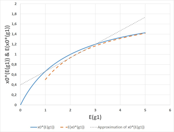
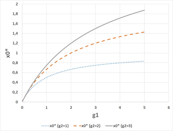
Observation:$x_0{}^{*}$ is a strictly increasing and strictly concave function of each g_i. From the Jensen inequality, it follows that increasing risk in g_i will reduce the expected value of $x_0{}^{*}$ . Compare Figure 1.

Second, the sensitivity analyses will concern these variables: $x_i{}^{*}={\lambda }_i{}^{*}=y_i{}^{*}={\mu }_i{}^{*},i=1,\mathrm{...},n$ . How do these variables change under the influence of changing elements in the game matrix?

Observation:$x_i{}^{*}={\lambda }_i{}^{*}=y_i{}^{*}={\mu }_i{}^{*}=g_i{}^{-1}{\left({\displaystyle \sum _{q=1}^n{g}_q{}^{-1}}\right)}^{-1},i=1,\mathrm{...},n$

Proof that $\frac{d{x}_i{}^{*}}{d{g}_i}<0\wedge \frac{d^2{x}_i{}^{*}}{d{g}_i{}^2}>0,i\in \left\{1,\mathrm{...},n\right\}$ .

$x_i{}^{*}=g_i{}^{-1}{\left({\displaystyle \sum _{q=1}^n{g}_q{}^{-1}}\right)}^{-1},i=1,\mathrm{...},n$ (2.3.8)

$\frac{d{x}_i{}^{*}}{d{g}_i}=-g_i{}^{-2}{\left({\displaystyle \sum _{q=1}^n{g}_q{}^{-1}}\right)}^{-1}+g_i{}^{-1}(-1){\left({\displaystyle \sum _{q=1}^n{g}_q{}^{-1}}\right)}^{-2}\left(-g_q{}^{-2}\right)$ (2.3.9)

$\frac{d{x}_i{}^{*}}{d{g}_i}=g_i{}^{-2}{\left({\displaystyle \sum _{q=1}^n{g}_q{}^{-1}}\right)}^{-1}\left(-1+g_i{}^{-1}{\left({\displaystyle \sum _{q=1}^n{g}_q{}^{-1}}\right)}^{-1}\right)$ (2.3.10)

$\frac{d{x}_i{}^{*}}{d{g}_i}=g_i{}^{-1}{x}_i{}^{*}\left(-1+x_i{}^{*}\right)$ (2.3.11)

$\left(g_i>0\right)\wedge \left(0<x_i{}^{*}<1\right)\Rightarrow \frac{d{x}_i{}^{*}}{d{g}_i}<0$ (2.3.12)

$\frac{d^2{x}_i{}^{*}}{d{g}_i{}^2}=-g_i{}^{-2}{x}_i{}^{*}\left(x_i{}^{*}-1\right)+g_i{}^{-1}\left(g_i{}^{-1}{x}_i{}^{*}\left(x_i{}^{*}-1\right)\right)\left(x_i{}^{*}-1\right)+g_i{}^{-1}{x}_i{}^{*}{g}_i{}^{-1}{x}_i{}^{*}\left(x_i{}^{*}-1\right)$ (2.3.13)

$\frac{d^2{x}_i{}^{*}}{d{g}_i{}^2}=-g_i{}^{-2}\left(x_i{}^{*}\left(x_i{}^{*}-1\right)-\left(x_i{}^{*}\left(x_i{}^{*}-1\right)\right)\left(x_i{}^{*}-1\right)-x_i{}^{*}{x}_i{}^{*}\left(x_i{}^{*}-1\right)\right)$ (2.3.14)

$\frac{d^2{x}_i{}^{*}}{d{g}_i{}^2}=-g_i{}^{-2}\left({\left(x_i{}^{*}\right)}^2-x_i{}^{*}-x_i{}^{*}\left({\left(x_i{}^{*}\right)}^2-2x_i{}^{*}+1\right)-{\left(x_i{}^{*}\right)}^2\left(x_i{}^{*}-1\right)\right)$ (2.3.15)

$\frac{d^2{x}_i{}^{*}}{d{g}_i{}^2}=-g_i{}^{-2}\left({\left(x_i{}^{*}\right)}^2-x_i{}^{*}-{\left(x_i{}^{*}\right)}^3+2{\left(x_i{}^{*}\right)}^2-x_i{}^{*}-{\left(x_i{}^{*}\right)}^3+{\left(x_i{}^{*}\right)}^2\right)$ (2.3.16)

$\frac{d^2{x}_i{}^{*}}{d{g}_i{}^2}=-g_i{}^{-2}\left(-2{\left(x_i{}^{*}\right)}^3+4{\left(x_i{}^{*}\right)}^2-2x_i{}^{*}\right)$ (2.3.17)

$\frac{d^2{x}_i{}^{*}}{d{g}_i{}^2}=2g_i{}^{-2}{x}_i{}^{*}\left({\left(x_i{}^{*}\right)}^2-2x_i{}^{*}+1\right)$ (2.3.18)

$\frac{d^2{x}_i{}^{*}}{d{g}_i{}^2}=2g_i{}^{-2}{x}_i{}^{*}{\left(x_i{}^{*}-1\right)}^2$ (2.3.19)

$\left(g_i\ne 0\right)\wedge \left(0<x_i{}^{*}<1\right)\Rightarrow \frac{d^2{x}_i{}^{*}}{d{g}_i{}^2}>0$ (2.3.20)

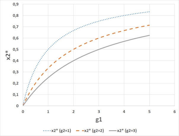
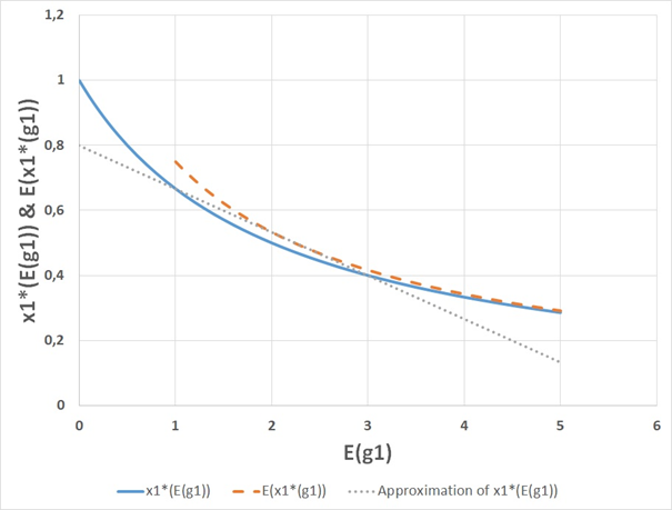
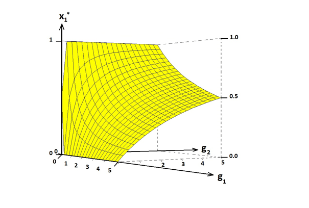
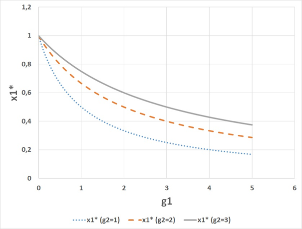
Observation:$x_i{}^{*}$ is a strictly decreasing and strictly convex function of g_i. From the Jensen inequality, it follows that increasing risk in g_i will increase the expected value of $x_i{}^{*}$ . Compare Figure 2.

Proof that $\frac{d{x}_k{}^{*}}{d{g}_i}>0\wedge \frac{d^2{x}_k{}^{*}}{d{g}_i{}^2}<0,i\in \left\{1,\mathrm{...},n\right\},k\in \left\{1,\mathrm{...},n\right\},i\ne k$ .

$x_k{}^{*}=g_k{}^{-1}{\left({\displaystyle \sum _{i=1}^n{g}_i{}^{-1}}\right)}^{-1}$ (2.3.21)

$\frac{d{x}_k{}^{*}}{d{g}_{i|i\ne k}}=g_k{}^{-1}\left(-1\right){\left({\displaystyle \sum _{i=1}^n{g}_i{}^{-1}}\right)}^{-2}\left(-g_i{}^{-2}\right)$ (2.3.22)

$\frac{d{x}_k{}^{*}}{d{g}_{i|i\ne k}}=g_k{}^{-1}{g}_i{}^{-2}{\left({\displaystyle \sum _{i=1}^n{g}_i{}^{-1}}\right)}^{-2}$ (2.3.23)

$\left(g_m>0,m=\mathrm{1...},n)\right)\Rightarrow \frac{d{x}_k{}^{*}}{d{g}_{i|i\ne k}}>0$ (2.3.24)

$\frac{d^2{x}_k{}^{*}}{d{g}_{i|i\ne k}{}^2}=g_k{}^{-1}\left(-2g_i{}^{-3}{\left({\displaystyle \sum _{i=1}^n{g}_i{}^{-1}}\right)}^{-2}+g_i{}^{-2}(-2){\left({\displaystyle \sum _{i=1}^n{g}_i{}^{-1}}\right)}^{-3}\left(-g_i{}^{-2}\right)\right)$ (2.3.25)

$\frac{d^2{x}_k{}^{*}}{d{g}_{i|i\ne k}{}^2}=2g_k{}^{-1}{g}_i{}^{-3}{\left({\displaystyle \sum _{i=1}^n{g}_i{}^{-1}}\right)}^{-2}\left(\left(g_i{}^{-1}\right){\left({\displaystyle \sum _{i=1}^n{g}_i{}^{-1}}\right)}^{-1}-1\right)$ (2.3.26)

$\frac{d^2{x}_k{}^{*}}{d{g}_{i|i\ne k}{}^2}=2g_k{}^{-1}{g}_i{}^{-1}{\left(x_i{}^{*}\right)}^2\left(x_i{}^{*}-1\right)$ (2.3.27)

$\left(g_m>0,m=1,\mathrm{...},n\right)\wedge \left(0<x_i{}^{*}<1\right)\Rightarrow \frac{d^2{x}_k{}^{*}}{d{g}_{i|i\ne k}{}^2}<0$ (2.3.28)

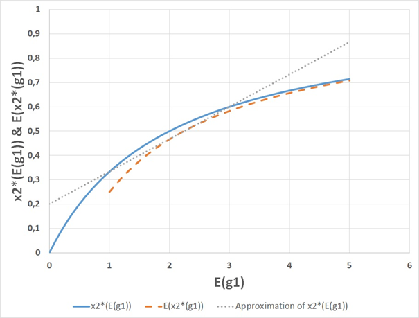
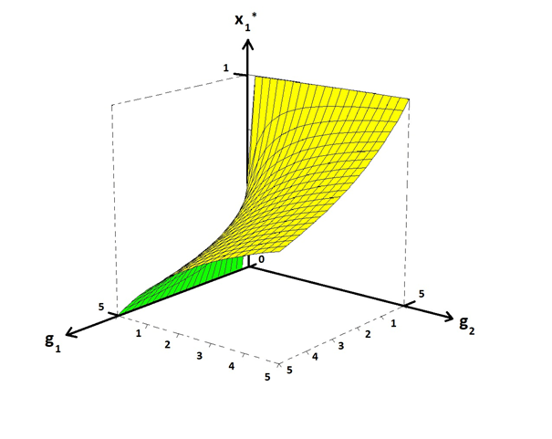
Observation:$x_k{}^{*}$ is a strictly increasing and strictly concave function of g_i. From the Jensen inequality, it follows that increasing risk in g_i will decrease the expected value of $x_k{}^{*}$ . Compare Figure 3.