The analysis in this paper shows that the fundamental theory of the CO₂ level in the atmosphere, under the influence of changing CO₂ emissions, can be modeled as a first order linear differential equation with a forcing function, describing industrial emissions.

Observations of the CO₂ level at the Mauna Loa CO₂ observatory and official statistics of global CO₂ emissions, from Edgar, the Joint Research Centre at the European Commission, are used to estimate all parameters of the forced CO₂ differential equation.

The estimated differential equation has a logical theoretical foundation and convincing statistical properties. It is used to reproduce the time path of the CO₂ data from Mauna Loa, from year 1990 to 2018, with very small errors. Furthermore, the differential equation shows that the global CO₂ level, without emissions, has a stable equilibrium at 280 ppm. This value has earlier been reported by IPCC as the pre-industrial CO₂ level.

The differential function is applied to derive four dynamic cases of the global CO₂ level, from the year 2020 until 2100, conditional on four different strategies concerning the development of global CO₂ emissions:

1. Emissions continue to increase according to the trend during 1990–2018
2. Emissions stay for ever at the 2020 level
3. Emissions are reduced with a linear trend to become zero year 2100
4. Emissions are reduced with a linear trend to become zero year 2050

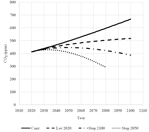
In case i., the CO₂ level year 2100 will be 688 ppm. In cases ii. and iii., the CO₂ levels in 2100 will be 517 ppm and 389 respectively. In case iv., the CO₂ level in 2050 is 408 ppm and then rapidly falls.

The global warming and CO₂ dynamics issue, for very good reasons, attracts considerable global interest. The climate of our planet is of key importance to all life. The author recommends the reader to study Ramade¹ in detail for a deep understanding of many of the connected issues and theories.

The first ambition is to understand the fundamental mechanisms of the dynamics of the CO₂ level of the atmosphere under the influence of global emissions.

We will investigate if it is possible to develop a theoretical mathematical model of the dynamics of CO₂. Such a model should be consistent with fundamental scientific principles. Furthermore, it should be possible to use the model to reproduce historical time series of empirical data. If such a model can be developed, it should be possible to use it also for predictions. Then, the most important application is to investigate how the global CO₂ level can be dynamically changed via different emissions strategies.

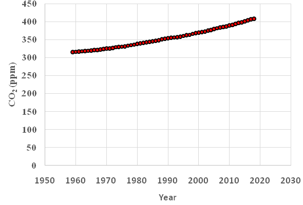
The CO₂ level of the atmosphere has been recorded since 1958, at the Mauna Loa observatory. See Tans and Keeling². The statistical tables are well documented and freely available via the internet. In Figure 1 the annual mean values of  CO₂ are shown. The web link connected to the reference provides access to all observations via a text file with instructions. In several cases, transformations between different physical units are necessary. O'Hara³ includes the relevant conversion factors.

Figure 1 CO₂ in the atmosphere, annual mean values, Mauna Loa, (ppm). Source: Tans and Keeling.²

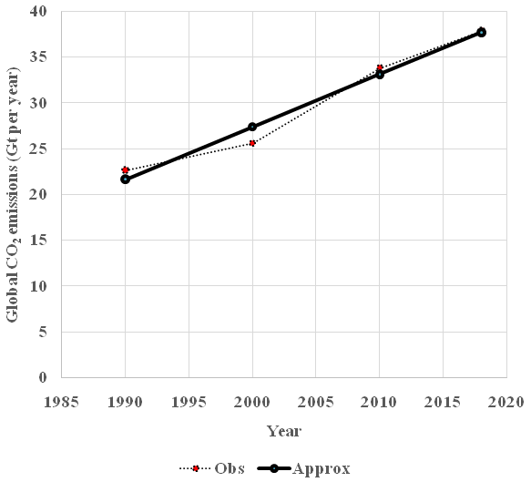
In Figure 2 we find observations of global CO₂ emissions from fossil fuels combustion and processes. These data come from European Commission.⁴ The observations from 1990, 2000, 2010 and 2018 have been used in the analysis of this paper. There are two reasons for this: First, emission data were only collected with ten year intervals during the early years. Second, sufficiently long time intervals are needed if we want to be able to estimate the changes of CO₂ in the atmosphere with sufficiently high precision. 

Figure 2 Obs=Observations of global CO₂ emissions from fossil fuels combustion and processes. Source: European Commission.⁴ Approx=Linear approximation via the least squares method, by the author of this paper. Compare equation (47).  Approx $=\text{}21.672+0.57366(Year-1990)$ . $R\approx 0.984$ .

In the estimations of a differential equation, the following three periods will be used: 1990–2000, 2000–2010 and 2010–2018. More details about these periods are found in Table 1.

The general theory of differential equations can be studied in Braun.⁵

Let us first consider the following differential equation. We will soon discover that it has to be adjusted in order to become relevant to the CO₂ problem.

$\stackrel{•}{x}=\frac{dx}{dt}=a_0$                                       (1)

$x=\text{}x(t)$ is the CO₂ level in the atmosphere as a function of time. $\stackrel{•}{x}=\frac{dx}{dt}$ is the change per time unit, or the time derivative, of $x$ . There are constant ”natural” emissions, from the oceans, volcanoes and other parts of the natural environment, greater than zero. $a_0>0$ . Hence, $\stackrel{•}{x}=\frac{dx}{dt}$ would be strictly positive and $x$ would increase over time, without bound, if nothing would stop that.

However, earlier CO₂ research has already shown that the CO₂ level has been stable during very long periods of time. Compare Ramade¹ and Solomon et al.⁶

Let us assume that the oceans (and, to some degree, other parts of the natural environment) absorb a part of the CO₂ in the atmosphere. Let us also assume that the absorbtion is proportional to the CO₂ level in the atmosphere, $x$ . This is a very reasonable assumption since the probability that a CO₂ molecule touches the surface of the sea is proportional to the CO₂ level in the atmosphere. Let the absorbtion be $-a_{x}x$ . Then, we have this differential equation of global CO₂:

$\stackrel{•}{x}=\frac{dx}{dt}=a_0+a_{x}x$                               (2)

Is there an equilibrium?

$\stackrel{•}{x}=\frac{dx}{dt}=a_0+a_{x}x=0$                          (3)

Yes, there is one and only one equilbrium.

$\left(\stackrel{•}{x}=0\right)\Rightarrow x=x_{eq}=\frac{-a_0}{a_x}>0$                     (4)

Is this equilibrium stable? Yes, if something disturbes $x$ so that $x<x_{eq}$ , then $\stackrel{•}{x}>0$ , which means that $x$ increases until $x=x_{eq}$ . If $x>x_{eq}$ , then $\stackrel{•}{x}<0$ , and $x$ decreases until $x=x_{eq}$ .

According to earlier research, the pre-industrial equilibrium level of CO₂ was 280 ppm (parts per million). Compare the IPCC report by Solomon et al.⁶ In this paper, we will find that the derived model confirms this finding. In other words, we will confirm that.

$x_{eq}=\frac{-a_0}{a_x}\approx 280$                                                           (5)

In order to determine the parameters of a function, it is necessary to have some variation in the data. In particular, when we want to determine the values of the parameters of the differential equation of $x$ , we can not do this if $x=x_{eq}$ all the time. In this respect, it is useful to observe that the industrial emissions of CO₂ during the latest decades have created earlier not available variation in $x$ . Let us regard global emissions of CO₂, after the industrial revolution, $\phi (t)$ , as a function of t. The emissions are added to the CO₂ in the atmosphere.

$\stackrel{•}{x}=a_0+a_{x}x+\phi (t)$                          (6)

Now, since we have access to empirical data for $\left(\stackrel{•}{x},\phi \right)$ in different time periods, we can estimate the parameters $\left(a_0,a_x\right)$ via the ordinary least squares method (regression analysis) in the following way:

$y(t)=\stackrel{•}{x}-\phi (t)=a_0+a_{x}x(t)$                          (7)

Table 1 includes the transformations of the available atmospheric CO₂ raw data to a time seriers of $\stackrel{•}{x}$ that will be used in the analysis. In a similar way, in Table 2 the global emission data is developed to time series data for $\phi$ .

In different statistical sources and equations, the CO₂ of the atmosphere is given in different units. Following the principles by O'Hara³, the following transformation rules have been applied: 1 ppm (CO₂) can be transformed to 2.13*3.664=7.80432 Gt CO₂. 1 ppm by volume of atmosphere CO₂=2.13 Gt C. 1 g C=0.083 mole CO₂=3.664 g CO_2.

Now, the data series developed in Table 1 and Table 2 are used to produce the regression data set found in Table 3.

Below, a very high level of detail in the calculations has been selected. The motivation is the following: The CO₂ dynamics and global warming issue is critical to the present global political debate. It is necessary that the reader can investigate and repeat all derivations without problems.

We want to determine the parameters $\left(a_0,a_x\right)$ in this function:

$y=a_0+a_{x}x$                                                                (8)

We minimize the sum of squares of the residuals:

$\underset{a_0,a_x}{\min }Z=\text{}{\displaystyle \sum _{i=1}^N{\left(y_i-a_0-a_x{x}_i\right)}^2}$                                            (9)

These are the first order optimum conditions:

$\{\begin{array}{c}\frac{dZ}{d{a}_0}=\text{}{\displaystyle \sum _{i=1}^N\left(2\left(y_i-a_0-a_x{x}_i\right)(-1)\right)}=0\\ \frac{dZ}{d{a}_x}=\text{}{\displaystyle \sum _{i=1}^N\left(2\left(y_i-a_0-a_x{x}_i\right)(-x_i)\right)}=0\end{array}$                             (10)

They are further developed:

$\{\begin{array}{c}\frac{dZ}{d{a}_0}=\text{}2{\displaystyle \sum _{i=1}^N\left(\left(a_0+a_x{x}_i-y_i\right)\right)}=0\\ \frac{dZ}{d{a}_x}=\text{}2{\displaystyle \sum _{i=1}^N\left(\left(a_0{x}_i+a_x{x}_i{}^2-x_i{y}_i\right)\right)}=0\end{array}$                                (11)

We also want to investigate if the derived solution gives a unique minimum:

$\frac{d^{2}Z}{d{a}_0{}^2}=2{\displaystyle \sum 1=2N}>0$                                                       (12)

$\frac{d^{2}Z}{d{a}_x{}^2}=2{\displaystyle \sum x^2}>0$                                                               (13)

$\Phi =\left|\begin{array}{cc}\frac{d^{2}Z}{d{a}_0{}^2}& \frac{d^{2}Z}{d{a}_{0}d{a}_x}\\ \frac{d^{2}Z}{d{a}_{x}d{a}_0}& \frac{d^{2}Z}{d{a}_x{}^2}\end{array}\right|=\left|\begin{array}{cc}2{\displaystyle \sum 1}& 2{\displaystyle \sum x}\\ 2{\displaystyle \sum x}& 2{\displaystyle \sum x^2}\end{array}\right|$                              (14)

$\Phi =4\left|\begin{array}{cc}N& {\displaystyle \sum x}\\ {\displaystyle \sum x}& {\displaystyle \sum x^2}\end{array}\right|=4\left(N{\displaystyle \sum x^2}-{\left({\displaystyle \sum x}\right)}^2\right)$                          (15)

$\Phi =4N^2\left(\frac{{\displaystyle \sum x^2}}{N}-{\left(\frac{{\displaystyle \sum x}}{N}\right)}^2\right)$                                              (16)

$\Phi =4N^2\left(E\left[x^2\right]-E{\left[x\right]}^2\right)$                                                 (17)

$\left(N>2\wedge Var(x)>0\right)\Rightarrow \Phi >0$                                           (18)

Hence, the second order conditions of a unique minimum are satisfied. The first order conditions give a unique minimum. The first order optimum conditions imply:

$\{\begin{array}{c}\text{}\left(N\right)a_0+\left({\displaystyle \sum x_i}\right)a_x=\left({\displaystyle \sum y_i}\right)\\ \left({\displaystyle \sum x_i}\right)a_0+\left({\displaystyle \sum x_i{}^2}\right)a_x=\left({\displaystyle \sum x_i{y}_i}\right)\end{array}$                                (19)

The parameters can be determined from this simultaneous equation system (Table 4):

$\left[\begin{array}{cc}N& {\displaystyle \sum x_i}\\ {\displaystyle \sum x_i}& {\displaystyle \sum x_i{}^2}\end{array}\right]\left[\begin{array}{c}{a}_0\\ a_x\end{array}\right]=\left[\begin{array}{c}{\displaystyle \sum y_i}\\ {\displaystyle \sum x_i{y}_i}\end{array}\right]$                                       (20)

The point $(a_0,a_x)$ is determined via Cramers rule:

$a_0=\frac{\left|\begin{array}{cc}{\displaystyle \sum y_i}& {\displaystyle \sum x_i}\\ {\displaystyle \sum x_i{y}_i}& {\displaystyle \sum x_i{}^2}\end{array}\right|}{\left|\begin{array}{cc}N& {\displaystyle \sum x_i}\\ {\displaystyle \sum x_i}& {\displaystyle \sum x_i{}^2}\end{array}\right|}\approx \frac{85248.955}{2081.723}\approx 40.951$                           (21)

$a_x=\frac{\left|\begin{array}{cc}N& {\displaystyle \sum y_i}\\ {\displaystyle \sum x_i}& {\displaystyle \sum x_i{y}_i}\end{array}\right|}{\left|\begin{array}{cc}N& {\displaystyle \sum x_i}\\ {\displaystyle \sum x_i}& {\displaystyle \sum x_i{}^2}\end{array}\right|}\approx \frac{-304.118}{2081.723}\approx -0.14609$                              (22)

If we express $\stackrel{•}{x}$ in the unit Gt CO₂/year, and $x$ in the unit ppm, we have this equation:

$\stackrel{•}{x}=40.951-0.14609x$                                                            (23)

What is the equilibrium value of $x$ , via the derived function, in case there are no emissions?

$\stackrel{•}{x}=\frac{dx}{dt}=a_0+a_x{x}_{eq}=0$                                                            (24)

$x_{eq}=\frac{-a_0}{a_x}\approx 280.31(ppm)$                                                    (25)

Note that this value confirms the ealier empirical finding by Solomon et al.⁶ If we express $\stackrel{•}{x}$ in the unit Gt CO₂/year, and $x$ in the unit Gt CO₂, we get the following differential equation (Figure 3). Note that the coefficient of $x$ has been divided by 2.13*3.664, namely by 7.80432  :

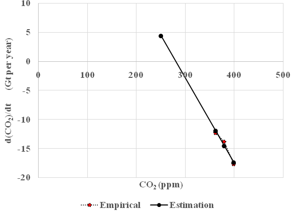
Figure 3 Determination of the global CO₂ differential equation via the empirical observations of CO₂ from Mouna Loa and the empirical observations of global CO₂ emissions. The estimated equilibrium value of CO₂ is 280 ppm, in case the global emissions of CO₂ are zero. This confirms the earlier findings. Compare Solomon et al.⁶ The estimated function is: 40.951 – 0.14609 * CO₂ (ppm). The multiple correlation coefficient R=0.977. Since the number of observations is limited, more detailed regression statistics will not be given here.

$\stackrel{•}{x}=40.951-0.0187191x$                                                   (26)

$x_{eq}=\frac{-40.951}{-0.0187191}\approx 2187.66(Gt)$                                    (27)

Now, the complete differential equation will be determined, giving the dynamic development of the CO₂ level in the amosphere as a function of the development of the global emissions.

This is the differential equation in general form:

$\stackrel{•}{x}=a_0+a_{x}x+\phi (t)$                                                (28)

We will consider the special case of emissions that grow with a linear trend, since that is supported by the available empirical data. (Note that the forcing function could be generalized to almost any form, if considered relevant.)

$\phi (t)=m_0+m_{1}t$                                                    (29)

The differential equation becomes:

$\stackrel{•}{x}-a_{x}x=a_0+m_0+m_{1}t$                                           (30)

Solution of the homogenous equation:

$\stackrel{•}{x_h}-a_x{x}_h=0$                                                           (31)

$x_h=A{e}^{st}$                                                                (32)

$\stackrel{•}{x_h}=sA{e}^{st}$                                                                (33)

$(s-a_x)x_h=0$                                                           (34)

$\left(x_h\ne 0\right)\Rightarrow s=a_x$                                                      (35)

$x_h(t)=A{e}^{a_{x}t}$                                                             (36)

Determination of the particular solution:

$x_p=k_0+k_{1}t$                                                            (37)

$\stackrel{•}{x_p}-a_x{x}_p=a_0+m_0+m_{1}t$                                         (38)

$k_1-a_x\left(k_0+k_{1}t\right)=a_0+m_0+m_{1}t$                                 (39)

$\{\begin{array}{c}{k}_1-a_x{k}_0=a_0+m_0\\ -a_x{k}_1=m_1\end{array}$                                                (40)

$\left(-a_x{k}_1=m_1\right)\Rightarrow k_1=\frac{-m_1}{a_x}$                                               (41)

$\left(k_1-a_x{k}_0=a_0+m_0\right)\wedge \left(k_1=\frac{-m_1}{a_x}\right)\Rightarrow \left(\frac{-m_1}{a_x}-a_x{k}_0=a_0+m_0\right)$                 (42)

$k_0=\frac{-\left(a_0+m_0+\frac{m_1}{a_x}\right)}{a_x}$                                                                       (43)

Determination of $\phi (t)=m_0+m_{1}t$

Now, in order to use the derived function for predictions, we estimate the parameters $\left(m_0,m_1\right)$ . We follow the same procedure as in the earlier section of this paper (Table 5 & 6).

The parameters can be determined from this simultaneous equation system:

$\left[\begin{array}{cc}N& {\displaystyle \sum t_j}\\ {\displaystyle \sum t_j}& {\displaystyle \sum t_j{}^2}\end{array}\right]\left[\begin{array}{c}{m}_0\\ m_1\end{array}\right]=\left[\begin{array}{c}{\displaystyle \sum {\phi }_j}\\ {\displaystyle \sum t_j{\phi }_j}\end{array}\right]$                                            (44)

The point $(m_0,m_1)$ is determined via Cramers rule:

$m_0=\frac{\left|\begin{array}{cc}{\displaystyle \sum {\phi }_j}& {\displaystyle \sum t_j}\\ {\displaystyle \sum t_j{\phi }_j}& {\displaystyle \sum t_j{}^2}\end{array}\right|}{\left|\begin{array}{cc}N& {\displaystyle \sum t_j}\\ {\displaystyle \sum t_j}& {\displaystyle \sum t_j{}^2}\end{array}\right|}\approx \frac{38403.096}{1772}\approx 21.672$                               (45)

$m_1=\frac{\left|\begin{array}{cc}N& {\displaystyle \sum {\phi }_j}\\ {\displaystyle \sum t_j}& {\displaystyle \sum t_j{\phi }_j}\end{array}\right|}{\left|\begin{array}{cc}N& {\displaystyle \sum t_j}\\ {\displaystyle \sum t_j}& {\displaystyle \sum t_j{}^2}\end{array}\right|}\approx \frac{1016.526}{1772}\approx 0.57366$                                    (46)

(The multiple correlation coefficient: R=0.984 )

$\phi (t)=21.672+0.57366t$                                                               (47)

$k_1=\frac{-m_1}{a_x}=\frac{-0.57366}{-0.0187191}\approx 30.646$                                                    (48)

$k_0=\frac{-\left(a_0+m_0+\frac{m_1}{a_x}\right)}{a_x}=\frac{-\left(40.951+21.672-30.646\right)}{-0.0187191}\approx 1708.27$                 (49)

$x(t)=A{e}^{-0.0187191t}+1708.27+30.646t$                                                     (50)

$x(0)=A+1708.27$                                                                                   (51)

$A=x(0)-1708.27$                                                                                   (52)

$A=354.39\cdot 2.13\cdot 3.664-1708.27$                                                             (53)

$A\approx 1057.52$                                                                                             (54)

$x(t)=1057.52e^{-0.0187191t}+1708.27+30.646t(Gt)$                               (55)

If the function is divided by (2.13*3.664), the unit becomes ppm.

$x(t)=135.50e^{-0.0187191t}+218.89+3.927t(ppm)$                                   (56)

In Figure 4 we find that the estimated function can reproduce the CO₂ observations from Mauna Loa extremely well. Most years during the period 1990 to 2018, the deviations are less than 1 ppm.

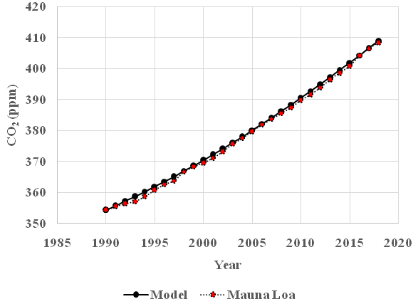
Figure 4 Mauna Loa= CO₂ observations from 1990 to 2018. Model= CO₂ prediction model. The empirical CO₂ observations from Mauna Loa, compare Figure 1 and the prediction according to the derived differential equation model are almost identical. The graph was derived with the following equation: $x(t)=135.50e^{-0.0187191t}+218.89+3.927t(ppm)$ .

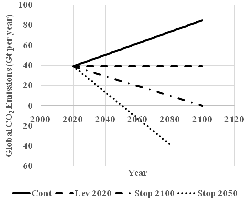
Now, the estimated differential equation will be used to predict the future development of the CO₂ level, conditional on the following four alternative global emission strategies:

Cont: During the period 2020 to 2100, the emissions continue to increase according to the trend estimated during the period 1990 to 2018.

Lev 2020: The emissions 2020 are estimated from the trend 1990 to 2018. Then, the emissions stay at that level until 2100.

Stop 2100: The emissions 2020 are estimated from the trend 1990 to 2018. Then, the emissions are reduced with a constant amount each year, such that the emissions are zero in 2100.

Stop 2050: The emissions 2020 are estimated from the trend 1990 to 2018. Then, the emissions are reduced with a constant amount each year, such that the emissions are zero in 2050.

In Figure 5 we see the graphs of the four emission scenarios and in Table 7. we find more details about the four scenarios.

Figure 5 Four different alternative scenarios for the future development of global CO₂ emissions, during the time interval 2020 to 2100. The emission level 2020 is estimated via the linear approximation based on data from the time interval 1990 to 2018. The scenarios are used to predict the future development of CO₂ in the atmosphere. Compare figure 6, Cont=The emissions continue to develop according to the trend during 1990 to 2018. Lev 2020=The emissions stay, for ever, at the level of 2020. Stop 2100=The emissions are reduced with the same amount each year, during the time interval 2020 until 2100. Then, the total emission is zero. Stop 2050=The emissions are reduced with the same amount each year, during the time interval 2020 until 2050. (Observation: The negative emissions after 2050 are technically possible but not necessarily optimal and relevant.)

The general principles derived and described in the earlier sections of this paper have been used to derive the equations of the CO₂ level that are consistent with the four different emission scenarios. The parameters are presented in Table 8 for the unit Gt, and in Table 9 for the unit ppm.

The developed model will now be used to investigate the dynamic effects of four different alternative scenarios for the future development of global CO₂ emissions, during the time interval 2020 to 2100. In Figure 5 we find the four emission scenarios. The predictions of the future CO₂ level, conditional on the different emission strategies, are found in Figure 6. The predictions function, (57) is used. Then, $t$ is defined according to the information in Table 7 and the parameter values $A,k_0,k_1$ from Table 9 are used. 

Figure 6 Four different alternative scenarios for the future development of CO₂ level in the atmosphere, during the time interval 2020 to 2100. The scenarios are conditional on the global emission scenarios found in figure 5. The emission level 2020 is estimated via the linear approximation based on data from the time interval 1990 to 2018. Cont=The emissions continue to develop according to the trend during 1990 to 2018.
Lev 2020=The emissions stay, for ever, at the level of 2020. Stop 2100=The emissions are reduced with the same amount each year, during the time interval 2020 until 2100. Then, the total emission is zero. Stop 2050=The emissions are reduced with the same amount each year, during the time interval 2020 until 2050. After 2050, the net emission is strictly negative and follows the same trend as before 2050. (Observation: The negative emissions after 2050 contribute to the dramatic fall of the CO₂level after 2050 in this scenario. If the emissions would be zero after 2050, the CO₂ level would converge to the pre-industrial level of 280 ppm. Alternative scenarios may easily be constructed.)

$x(t)=A{e}^{-0.0187191t}+k_0+k_{1}t(ppm)$                                                     (57)

Now, it is possible to understand the fundamental mechanisms of the dynamics of the CO₂ level of the atmosphere, under the influence of global emissions.

A theoretical mathematical model of the dynamics of CO₂ has been developed. This model is consistent with fundamental scientific principles. Furthermore, we can use the model to reproduce historical time series of empirical data. We can even use the model to calculate the pre-industrial level of CO₂ and discover that the calculated equilibrium value is consistent with earlier research findings. The model can also be used for Predictions. We have investigated how the global CO₂ level can be dynamically changed via different emissions strategies. Detailed predictions of possible future developments have been produced and described.

The CO₂ and global warming topic is central to the present global political agenda. It is necessary to create a fundamental understanding of the principles and methods that can be used to handle the problems and to stabilize our global climate. The model developed in this paper can hopefully make it possible for a large part of the human population to really understand how the CO₂ dynamics and emissions are connected. Without this fundamental understanding, it is difficult to convince critical persons that large investments in emission reductions may be necessary in order to stabilize the global climate.

The model developed in this paper should be possible to understand, investigate and to reproduce, in every detail by every person that has a PhD or masters degree in engineering, mathematics, mathematical statistics or mathematical economics. Earlier models presented on similar topics are not presented with all the details. Completeness and transparancy are necessary for complete understanding and acceptance.

According to the Occams razor, a scientific model should not be more complicated than necessary. In this paper, a differential equation is developed that is only based on very fundamental principles from physical science and mathematics. Two highly reliable sources of empirical data have been used to estimate the parameters. In the analysis, we have seen that a first order differential equation with emission forcing has been able to explain the development of the dynamics of the CO₂ level in the atmosphere, with very high precision. Furthermore, the function shows that the CO₂ equilibrium level, before the industrial revolution, should be 280 ppm, which confirms earlier empirical research. According to the opinion of the author, it is hardly possible to develop a more simple scientific model that explains the CO₂ dynamics in a better way.

Finally, the author hopes that the new model will be used to optimize and control global emission reductions, in order to give our planet the optimal climate.

None.

None.

The author declares that there was no conflict of interest.

1. Ramade F. Ecology of Natural Resources. New York: Wiley; 1984. p. 231.
2. Tans P, Keeling R. Trends in Atmospheric Carbon Dioxide. NOAA Research. 2019.
3. O'Hara Fred Jr Carbon Dioxide and Climate, 3rd edition.Tennessee: Oak Ridge; 1990.
4. European Commission. Joint Research Centre, Edgar–Emission database for global atmospheric research. 2019.
5. Braun M. Differential Equations and Their Applications. Applied Mathematics Sciences, Springer. 1986;15:546.
6. Solomon S, Qin D, Manning M, et al. Climate Change 2007-The Physical Science Basis. Contribution of Working Group I to the Fourth Assessment Report of the Intergovernmental Panel on Climate Change. UK: Cambridge University Press; 2007.