A general spatial fire brigade unit network density optimization problem has been solved. The distance to a particular road, from a fire station, is approximated as a continuous variable. It is proved, via integral convolution, that the probability density function of the total travel time, PDFT, is triangular. The size of the fire, when it stopped, is a function of the time it takes until the fire brigade reaches the fire location. An explicit continuous function for the expected total cost per square kilometer, based on the cost per fire station, the PDFT, the exponential fire cost function parameters, the distance between fire stations, and the speed of fire engines, is derived. It is proved that the optimal distance between fire brigade unit positions, OFD, which minimizes the total expected cost, is unique. Then, the OFDs are replaced by integers, OFDIs, for different parameter assumptions. In this process, also the optimal expected total costs are determined. It is proved that the OFD is a strictly decreasing function of the expected number of fires per area unit, a strictly increasing function of the speed of the fire engines, a strictly decreasing function of the parameters of the exponential fire cost function, and a strictly increasing function of the cost per fire station. These effects of parameter changes are also illustrated via graphs in the numerical section.

Keywords: OFD, fire, road, weather, optimization

Wild fire’s cause tremendous problems in many countries. In recent years, global warming has been considered as a possible reason why the burned areas are increasing. Williams et al.,¹ write that the annual wildfires in California have increased about five times since the early years of the 1970s. They describe how global warming, caused by humans, increases the temperature. As a consequence, the fuel becomes drier than in the past. Heat, dry fuels and strong winds, in combination, make the wild fires much worse than earlier. Mohammadi et al.,² investigate how climate factors influence the size of wildfires. They develop a multivariate nonlinear fire size model and estimate the parameters based on data from documented wildfires in Czech Republic. The size of a fire increases as a function of the air temperature and the wind speed, and decreases as a function of the relative humidity. Higher air temperatures, higher wind speeds and lower relative humidity, at least locally, can follow from global warming. This means that larger wild fires can be expected if the global warming continues. Global warming is a process that may be predicted and adjusted via CO₂ emission control. Still, even with dramatic emission reductions, the temperature can be expected to increase during many years, as described by Lohmander.³ Lohmander⁴ has investigated the burned areas in 29 countries with very different conditions. He found that the relative burned areas in different countries can be explained via a nonlinear function based on average temperatures and proxy variables representing firefighting capacities and expected distances between fire stations and wild fires. The statistical analysis showed that the relative burned areas are increasing functions of average temperatures and expected distances between fire stations and fire locations, and decreasing functions of fire fighting capacities. All parameters were strongly significant. Lohmander⁵ investigated the optimal forestry, infrastructure and fire management problem. With general functions, he derived optimal solutions that showed the optimal directions of different management changes under the influence of global warming.

In many cases, the speed of fire fighting is very important. For this reason, Kolesar⁶ and Kolesar et al.,⁷ estimate different functions for fire company travel times in New York. In another study, Kolesar et al.,⁸ are interested in the spatial density of firefighting companies. The find that the average fire engine company response distance can be modeled as an inverse square root function. They write that such functions can be useful in order to find optimal resource allocations. A similar topic and interest can be found in Sozuki et al.⁹ They want to optimize the locations of fire departments. In order to do this, they minimize average response times. These ideas have some connections to the new model and results that will be derived in this paper. In this paper, however, the average distances and average travel times are not studied. The reason is that the sizes and costs of wildfires usually grow as nonlinear, strictly convex, functions of time, at least during the early history of a particular fire. If we are interested to optimize the expected total result, the nonlinearities of the fire size and fire cost functions have to be explicitly taken into consideration when fire engine locations are optimized, which follows from the Jensen inequality. In remote areas, water bombing airplanes are necessary resources. The optimal use of such resources and optimal international cooperation in this area has been analyzed via stochastic dynamic programming, by Lohmander.¹⁰ In many cases, conditions of relevance to fire management change rapidly. For instance, in Canada and Russia, the probabilities of severe wild fires are very low during the winter, when snow covers the forests. In the summer, the conditions may rapidly change. During hot and dry periods, fires easily start. If the winds are strong, the fires may also rapidly grow. It is obviously important to investigate if it is possible to adapt the fire management decisions to different conditions.

If we predict that we will approach a hot and dry period with strong winds, it is almost surely rational to be more prepared to rapidly respond to possible fires, than if we expect rain storms. A central question is then: In what ways can we rapidly become more prepared to fight fires? If we expect the next days to be critical, with hot dry weather and strong winds, there is no time to improve roads, change forest management strategies and so on. On the other hand, we may move fire engines and other mobile resources, including man power, to optimal positions. Since we do not know exactly where the fires will start, we cannot go there before they have started. However, we can increase the number of units that are prepared and we can distribute them over the total area. In other words, we can increase the density of the defense against wild fire. We can decrease the distance between fire stations. (In this context, “fire station” denotes a firefighting unit, including a fire engine, manpower and other resources.) The ambition in this paper is to give a general solution to the optimal spatial fire brigade unit network density problem. It is important to know how the optimal solution depends on different conditions. The size of a wild fire changes over time. A typical wild fire starts in some spatially random position. At some point in time, it is discovered. Then perhaps with some delay, the closest fire brigade unit starts to move to the fire. During the travel time, the fire grows. In extreme cases, it is possible that the travel time is very long and most of the fuel is consumed before the fire is stopped. Normally, however, the travel time is rather short and the fire grows more and more rapidly during the time of interest, namely the time it takes before the fire has been stopped. For these reasons, the fire cost is assumed to be an exponential function of time.

We will investigate the problem in the most general way. We consider a uniform spatial structure that can easily be applied in most countries and types of regions. In fact, the general method can be applied in a city or in a less populated forest region. A fire can start anywhere. The probability is the same in every part of the region. This is usually a reasonable approximation of reality when we consider forest fires started by thunder storms and similar natural phenomena. Hence, a spatially uniform wild fire probability density function is applied. When a fire has been discovered, the fire brigade unit with the shortest travel distance to the fire is engaged. The road network contains roads from South to North and West to East. The cost of the fire, when it stopped, is a function of the time it takes until the fire brigade reaches the fire location. The probability density function of the travel time will be derived, since it is needed in the calculation of the expected cost. That cost is also needed in order to optimize the density of the fire defense. A function for the expected total cost per area unit, based on the cost per fire station, the PDFT, the exponential fire cost function parameters, the distance between fire stations, and the speed of fire engines, will be derived. Maybe, there are several local optima? The qualitative properties of the optimal solution(s) have to be studied, since it is necessary to know if the derived solution(s) also represent(s) the globally best solution(s).

Here, a general spatial fire brigade unit network density optimization problem will be solved. The optimal distance between fire brigade units positions is denoted OFD. In the analysis, the distance is denoted by x and the optimal distance, OFD, is denoted by x^* in order to make the exposition easier to follow.

The optimization problem

In equation (1), we maximize the expected total value per area unit.

$\underset{x}{\max }N(x)=-c_x{x}^{-2}+\left(N_0-pE\left(C\left(y\left(x\right)\right)\right)\right)$   (1)

N(x) is the Net value of the region under consideration, per square kilometer, as a function of x, the distance between fire stations, in kilometers. The cost per fire station is c_x (USD/Day). N₀ denotes the value of the area in case wild fires never occur and the number of fire stations would be zero. The probability that a wild fire occurs within a particular square kilometer, a particular day, is p. The travel time for a fire engine, from the fire to the closest fire station, is y. C is the cost of a fire and E(C) is the expected value of C. In this analysis, we do not consider cases where a particular fire brigade unit simultaneously is engaged in several fires. In multiple fire events, we rely on assistance from neighbor fire stations and water bombing airplanes. In equation (2), L(x) is defined as the expected total cost of fire stations and fires.

$L(x)=c_x{x}^{-2}+pE\left(C\left(y\left(x\right)\right)\right)$   (2)

We may express the maximization problem as in equation (3).

$\underset{x}{\max }N\left(x\right)=N_0-L\left(x\right)$   (3)

We may understand L(x) as the difference between N₀ and N(x). Compare (4).

$L\left(x\right)=N_0-N\left(x\right)$   (4)

Now, we will focus on the minimization of L(x), as in (5).

$\underset{x}{\min }L\left(x\right)=\left(c_x{x}^{-2}+pE\left(C\left(y\left(x\right)\right)\right)\right)$   (5)

We let stars indicate optimal values.

$L^{*}=\underset{x}{\min }L\left(x\right)=L\left(x^{*}\right)$   (6)

We simplify the notation this way:

$M(x)=E\left(C\left(y\left(x\right)\right)\right)$   (7)

The first order optimum condition is:

$\frac{dL}{dx}=-2c_x{x}^{-3}+p\frac{dM}{dx}=0$   (8)

In case we can show that the second order minimum condition (9) is satisfied, then we have a unique minimum (10). However, this will be investigated in detail before we can be sure.

$\frac{d^{2}L}{d{x}^2}=6c_x{x}^{-4}+p\frac{d^{2}M}{d{x}^2}>0$   (9)

$\left(c_x>0,p\ge 0,0<x^{*}<\infty ,\frac{d^{2}M}{d{x}^2}\ge 0\right)\Rightarrow \left(\exists x^{*}\wedge x^{*}unique\right)$   (10)

If we have a unique optimal solution, then the optimal solution may hopefully be obtained from the first order optimum condition:

$\left(\frac{dL}{dx}=0\right)\Rightarrow \left(p\frac{dM}{dx}=2c_x{x}^{-3}\right)$   (11)

The expected cost as a function of x

We consider a road network with parallel two-way roads, from West to East (WE) (and the opposite direction, EW) and from South to North (SN) (and the opposite direction, NS). (Of course, the model is still relevant even if the directions are quite different, as long as the different directions are perpendicular to each other.) The total area of the road network is very large. In order to simplify the exposition and the derivations, we consider it to be infinite. Hence, we do not have to consider special cases along the boundaries of the total network. Fire stations are located with constant distances between them, along the West to East roads (WE) and along the South to North roads (SN). If we consider four neighbor fire stations, they are found in the different corners of a square, defined by roads that together form a perfect square. The distances between the closest stations are x. The distances between parallel roads are constant and much shorter than x. To simplify the analysis, we use the approximation that these distances are zero. The distance from an arbitrary point to the closest station, in direction WE or EW is less than or equal to x/2. The distance from an arbitrary point to the closest station in direction SN or NS is also less than or equal to x/2. If a fire starts in a point Q, then the fire brigade that has the shortest total distance to Q travels to Q. The fire brigade has to follow the roads in the network. The probability that a wildfire starts is the same everywhere, which means that the probability density is constant. Hence, a spatially uniform wild fire probability density function is applied. The expected travel distance from the closest station to Q, in the EW or WE direction, is x/4, and the expected travel distance in the SN or NS direction, is x/4. Hence, the expected total travel distance from the closest station to Q is x/2. We assume that the travel time is proportional to the travel distance. This is approximately correct if vehicle acceleration and retardation time intervals only represent very small parts of the total travel time.

T is the time it takes to go between two neighbor fire brigade unit locations. x (km) is the distance and s (km/min) is the speed. Note that the speed, s, depends on the properties of the fire engines and the roads. It would be possible to extend the analysis by also optimizing the fire engine speed and the road quality. The unit of T is minutes.

$T=\frac{x}{s}$   (12)

We assume that the travel time in direction WE or EW is y₁ and the travel time in direction SN or NS is y₂. The uniform probability density function of the travel time from the closest fire brigade unit to the fire, in the WE or WE direction can be expressed as:

$f_1\left(y_1\right)=\{\begin{array}{ccc}0& for& y_1<0\\ \left(2/T\right)& for& 0\le y_1\le (T/2)\\ 0& for& \left(T/2\right)\le y_1\end{array}$   (13)

Furthermore, the uniform probability density function of the travel time from the closest fire brigade unit to the fire, in the SN or NS direction, y₂, can be expressed as:

$f_2\left(y_2\right)=\{\begin{array}{ccc}0& for& y_2<0\\ \left(2/T\right)& for& 0\le y_2\le \left(T/2\right)\\ 0& for& \left(T/2\right)\le y_2\end{array}$   (14)

The total travel time, y, is y₁ + y₂. The probability density function of y is f(y). This can be determined via convolution based on the probability density functions of and y₁ and y₂, namely f₁(y₁) and f₂(y₂). Now, via convolution, we can determine the probability density function of the total travel time y, via the following function:

$f\left(y\right)={\displaystyle \underset{0}{\overset{T}{\int }}{f}_1\left(y_1\right)}{f}_2\left(y-y_1\right)d{y}_{1}0\le y\le T$   (15)

Inspection reveals that the probability density function of the total travel time can be explicitly described as:

$f\left(y\right)=\{\begin{array}{cccc}0& y<0& & \\ \left(4/T^2\right)y& 0\le y<\left(T/2\right)& & \\ (4/T)-\left(4/T^2\right)y& \left(T/2\right)\le y\le T& & \\ 0& T<y& & \end{array}$   (16)

Hence, the probability density is a “triangular” function of total travel time. It is important to determine the optimal distance between fire stations under different conditions. In other words, we want to optimize x as a function of relevant parameters. We are interested to minimize the expected value of the expected total cost of the complete system. In this process, it is necessary to calculate the expected cost of the fire(s) as a function of x. The expected cost of a fire can be determined via two functions, namely the cost as a function of total travel time and the probability density function of total travel time. This is found here:

$E_1\left(x\right)=E\left(C\left(y\left(T\left(x\right)\right)\right)\right)={\displaystyle \underset{0}{\overset{T(x)}{\int }}C(y)f\left(y;T\left(x\right)\right)dy}$   (17)

Using the derived probability density function of total travel time, we get the following expression for the expected cost:

$E_2={\displaystyle \underset{0}{\overset{\left(T/2\right)}{\int }}C(y)\left(4/T^2\right)ydy}+{\displaystyle \underset{\left(T/2\right)}{\overset{T}{\int }}C(y)\left(4/T-\left(4/T^2\right)y\right)dy}$   (18)

The fire cost function is approximated as an exponential function of total travel time. Of course, the analysis in this paper can also be adjusted to other functional forms of fire cost functions, if locally relevant empirical data motivate that.

$C(y)=a{e}^{by}$   (19)

With the selected fire cost function, we get the following expression for the expected fire cost:

$E_2={\displaystyle \underset{0}{\overset{\left(T/2\right)}{\int }}a{e}^{by}\left(4/T^2\right)ydy}+{\displaystyle \underset{\left(T/2\right)}{\overset{T}{\int }}a{e}^{by}\left(4/T-\left(4/T^2\right)y\right)dy}$   20)

$E_2=a\left({\displaystyle \underset{0}{\overset{\left(T/2\right)}{\int }}{e}^{by}\left(4/T^2\right)ydy}+{\displaystyle \underset{\left(T/2\right)}{\overset{T}{\int }}{e}^{by}\left(4/T-\left(4/T^2\right)y\right)dy}\right)$   (21)

Integration section

In order to calculate the expressions, we need the following integral in several places:

${\displaystyle \int y{e}^{by}dy}$   (22)

From the Leibniz product rule, we know that:

$\frac{d\left(u(y)v(y)\right)}{dy}=\frac{du}{dy}v(y)+u(y)\frac{dv}{dy}$   (23)

We may integrate the left hand and the right hand sides of the equality.

${\displaystyle \int \frac{d\left(u(y)v(y)\right)}{dy}}dy={\displaystyle \int \frac{du}{dy}v(y)}dy+{\displaystyle \int u(y)\frac{dv}{dy}}dy$   (24)

$u(y)v(y)={\displaystyle \int \frac{du}{dy}v(y)}dy+{\displaystyle \int u(y)\frac{dv}{dy}}dy$   (25)

$Letu(y)=y,v(y)=b^{-1}{e}^{by}$   (26)

$\frac{du}{dy}=1\wedge \frac{dv}{dy}=e^{by}$   (27)

Then, we get:

$y{b}^{-1}{e}^{by}={\displaystyle \int b^{-1}{e}^{by}}dy+{\displaystyle \int y{e}^{by}}dy$   (28)

$b^{-1}y{e}^{by}=b^{-1}{\displaystyle \int e^{by}}dy+{\displaystyle \int y{e}^{by}}dy$   (29)

This may be expressed as:

${\displaystyle \int y{e}^{by}}dy=b^{-1}\left(y{e}^{by}-{\displaystyle \int e^{by}}dy\right)$   (30)

Then we have the solution:

${\displaystyle \int y{e}^{by}}dy=\left(b^{-1}y-b^{-2}\right)e^{by}$   (31)

Test:

$\frac{d\left(\left(b^{-1}y-b^{-2}\right)e^{by}\right)}{dy}=b^{-1}{e}^{by}+\left(b^{-1}y-b^{-2}\right)b{e}^{by}=y{e}^{by}Q.E.D.$   (32)

Explicit solution

In equation (33), we utilize the solution (31).

$E_2=\frac{4a}{T^2}\left({\left(b^{-1}y-b^{-2}\right)e^{by}|}_0^{\left(\frac{T}{2}\right)}\right)+\frac{4a}{T}\left({b^{-1}{e}^{by}|}_{\left(\frac{T}{2}\right)}^T\right)-\frac{4a}{T^2}\left({\left(b^{-1}y-b^{-2}\right)e^{by}|}_{\left(\frac{T}{2}\right)}^T\right)$   (33)

This is developed to (34).

$E_2=\frac{4a}{T^2}\left(\frac{T{e}^{b\frac{T}{2}}}{2b}-\frac{e^{b\frac{T}{2}}}{b^2}+\frac{1}{b^2}\right)+\frac{4a}{T}\left(\frac{e^{bT}}{b}-\frac{e^{b\frac{T}{2}}}{b}\right)-\frac{4a}{T^2}\left(\frac{T{e}^{bT}}{b}-\frac{e^{bT}}{b^2}-\frac{T{e}^{b\frac{T}{2}}}{2b}+\frac{e^{b\frac{T}{2}}}{b^2}\right)$   (34)

Then, we get equation (35).

$\begin{array}{l}{E}_2=\frac{2a}{bT}{e}^{b\frac{T}{2}}-\frac{4a}{b^2{T}^2}{e}^{b\frac{T}{2}}+\frac{4a}{b^2{T}^2}+\frac{4a}{bT}{e}^{bT}-\frac{4a}{bT}{e}^{b\frac{T}{2}}\\ -\frac{4a}{bT}{e}^{bT}+\frac{4a}{b^2{T}^2}{e}^{bT}+\frac{2a}{bT}{e}^{b\frac{T}{2}}-\frac{4a}{b^2{T}^2}{e}^{b\frac{T}{2}}\end{array}$   (35)

After some elimination, we obtain equation (36), which is then simplified to (37).

$E_2=\frac{4a}{b^2{T}^2}\left(e^{bT}-2e^{b\frac{T}{2}}+1\right)$   (36)

$E_2=\frac{4a{\left(e^{b\frac{T}{2}}-1\right)}^2}{b^2{T}^2}$   (37)

We may also express the expected cost as a function of x and s, which is found in (38).

$\left(T=\frac{x}{s}\right)\Rightarrow E_2=\frac{4a{s}^2{\left(e^{b\frac{x}{2s}}-1\right)}^2}{b^2{x}^2}$   (38)

The new variable introduced in equation (39) represents a way to simplify the following expressions. This way, we get (40).

$\phi =\frac{bT}{2}$   (39)

$E_2=a{\left(\frac{e^{\phi }-1}{\phi }\right)}^2$   (40)

In order to solve the optimization problem, we need the first order derivative found in (41).

$\frac{d{E}_2}{d\phi }=2a\left(\frac{e^{\phi }-1}{\phi }\right)\left(\frac{e^{\phi }\phi -e^{\phi }+1}{{\phi }^2}\right)$   (41)

Since we are interested in the sign of (41), we simplify the analysis further. We introduce a new function (43), also found in (42).

$\frac{d{E}_2}{d\phi }=2a\left(\frac{e^{\phi }-1}{\phi }\right)\left(\frac{\beta \left(\phi \right)}{{\phi }^2}\right)$   (42)

$\beta \left(\phi \right)=e^{\phi }\phi -e^{\phi }+1$   (43)

$\beta \left(0\right)=0$   (44)

$\frac{d\beta }{d\phi }=e^{\phi }\phi$   (45)

$\left(\phi >0\right)\Rightarrow \frac{d\beta }{d\phi }=e^{\phi }\phi >0$   (46)

As we see in (47), the sign of the function is strictly positive.

$\left(\phi >0\right)\Rightarrow \beta \left(\phi \right)>0$   (47)

Thanks to the observation (47), we can determine the sign of the derivative (48).

$\left(a>\wedge \phi >0\right)\Rightarrow \frac{d{E}_2}{d\phi }>0$   (48)

In (49), (50) and (51), more results follow.

$\left(a>\wedge \phi >0\right)\Rightarrow \left(\frac{d{E}_2}{dT}>0\wedge \frac{d{E}_2}{db}>0\right)$   (49)

$\frac{d{E}_1}{dx}=\frac{d{E}_2}{dT}\frac{dT}{dx}=\frac{d{E}_2}{dT}{s}^{-1}>0$   (50)

$\frac{d{E}_1}{ds}=\frac{d{E}_2}{dT}\frac{dT}{ds}=\frac{d{E}_2}{dT}\left(-x{s}^{-2}\right)<0$   (51)

Now we know that the expected fire cost is a strictly increasing function of the total travel time between neighbor fire stations, the two exponents in the fire cost function and the distance between fire stations. The expected fire cost is a strictly decreasing function of the speed of the fire engines.

Investigation of the second order derivative

We want to make sure that a solution to the first order optimum condition (8) really is a minimum. If possible, we also want to know if a solution is a global minimum. This investigation is made in several steps, with new partial functions, as illustrated in equations (53) to (68).

$\frac{d{E}_2}{d\phi }=2a\left(\frac{e^{\phi }-1}{\phi }\right)\left(\frac{e^{\phi }\phi -e^{\phi }+1}{{\phi }^2}\right)$   (52)

$\frac{d^2{E}_2}{d{\phi }^2}=a{\phi }^{-4}\left(2e^{2\phi }\left(2{\phi }^2-4\phi +3\right)-2e^{\phi }\left({\phi }^2-4\phi +6\right)+6\right)$   (53)

$\frac{d^2{E}_2}{d{\phi }^2}=a{\phi }^{-4}\gamma \left(\phi \right)$   (54)

$\gamma \left(\phi \right)=2e^{2\phi }\left(2{\phi }^2-4\phi +3\right)-2e^{\phi }\left({\phi }^2-4\phi +6\right)+6$   (55)

$\gamma \left(0\right)=0$   (56)

$\frac{d\gamma \left(\phi \right)}{d\phi }=e^{\phi }\left(4e^{\phi }\left(2{\phi }^2-2\phi +1\right)-2\left({\phi }^2-2\phi +2\right)\right)$   (57)

$\frac{d\gamma \left(0\right)}{d\phi }=0$   (58)

$\frac{d\gamma \left(\phi \right)}{d\phi }=e^{\phi }\theta \left(\phi \right)$   (59)

$\theta \left(\phi \right)=4e^{\phi }\left(2{\phi }^2-2\phi +1\right)-2\left({\phi }^2-2\phi +2\right)$   (60)

$\theta \left(0\right)=0$   (61)

$\frac{d\theta \left(\phi \right)}{d\phi }=4e^{\phi }\left(2{\phi }^2+2\phi -1\right)-4\left(\phi -1\right)$   (62)

$\frac{d\theta \left(0\right)}{d\phi }=0$   (63)

$\frac{d{\theta }^2\left(\phi \right)}{d{\phi }^2}=4\left(e^{\phi }\left(2{\phi }^2+6\phi +1\right)-1\right)$   (64)

$\left(\phi \ge 0\right)\Rightarrow \frac{d{\theta }^2\left(\phi \right)}{d{\phi }^2}>0$   (65)

$\left(\left(\theta \left(0\right)=0\right)\wedge \left(\frac{d\theta \left(0\right)}{d\phi }=0\right)\wedge \left({\frac{d{\theta }^2\left(\phi \right)}{d{\phi }^2}|}_{\phi \ge 0}>0\right)\right)\Rightarrow \left({\theta \left(\phi \right)|}_{\phi >0}>0\right)$   (66)

$\left({\theta \left(\phi \right)|}_{\phi >0}>0\right)\Rightarrow \left({\gamma \left(\phi \right)|}_{\phi >0}>0\right)$   (67)

$\left({\gamma \left(\phi \right)|}_{\phi >0}>0\wedge a>0\right)\Rightarrow \left({\frac{d^2{E}_2}{d{\phi }^2}|}_{\phi >0}>0\right)\Rightarrow \left({\frac{d^{2}M}{d{x}^2}|}_{x>0}>0\right)$   (68)

Now, we know that the expected fire cost really is a strictly convex function of the distance between fire stations.

Comparative statics analysis

Now, we want to know how the optimal decisions are affected by possible parameter changes. We start with the first order optimum condition (69).

$\frac{dL}{dx}=-2c_x{x}^{-3}+p\frac{dM}{dx}=0$   (69)

We differentiate the first order optimum condition with respect to the optimal value of x and the probability p.

$d\left(\frac{dL}{dx}\right)=\frac{d^{2}L}{d{x}^2}d{x}^{*}+\frac{d^{2}L}{dxdp}dp=0$   (70)

$\frac{d^{2}L}{d{x}^2}d{x}^{*}=-\frac{d^{2}L}{dxdp}dp$   (71)

$\frac{d{x}^{*}}{dp}=-\frac{\left(\frac{d^{2}L}{dxdp}\right)}{\left(\frac{d^{2}L}{d{x}^2}\right)}$   (72)

$\frac{d^{2}L}{d{x}^2}=6c_x{x}^{-4}+p\frac{d^{2}M}{d{x}^2}$   (73)

$\left(c_x>0\wedge x<\infty \wedge p\ge 0\wedge \frac{d^{2}M}{d{x}^2}>0\right)\Rightarrow \left(\frac{d^{2}L}{d{x}^2}>0\right)$   (74)

$\frac{d^{2}L}{dxdp}=\frac{dM}{dx}$   (75)

$\left(\frac{d{E}_1}{dx}>0\right)\Rightarrow \left(\frac{dM}{dx}>0\right)\Rightarrow \left(\frac{d^{2}L}{dxdp}>0\right)$   (76)

$\left(\frac{d^{2}L}{d{x}^2}>0\wedge \frac{d^{2}L}{dxdp}>0\right)\Rightarrow \left(\frac{d{x}^{*}}{dp}<0\right)$   (77)

Hence, as expected, we see that the optimal distance x is a strictly decreasing function of the probability p. It is obviously more important to have shorter distances to go to reach the fires if the probability of fires increases.

With the corresponding procedure, it can also be proved that:

$\frac{d{x}^{*}}{da}<0\wedge \frac{d{x}^{*}}{db}<0\wedge \frac{d{x}^{*}}{d{c}_x}>0\wedge \frac{d{x}^{*}}{ds}>0$   (78)

We may now summarize the general results: If the probability that a fire starts, p, increases, then the optimal distance between fire stations decreases. The optimal distance also decreases in case the fire cost function, C(y), increases, via one or two of the parameters a and b. The optimal distance between fire stations increases if the cost per fire station increases. If the speed of fire engines increases, because of improved fire engines and/or because of better roads, then the optimal distance between fire stations increases.

Numerical results

In the earlier section, it was proved that the optimal distance between fire brigade unit positions, x, which minimizes the total expected cost, is unique. x is a continuous variable and optimal solutions are usually not integers. The optimal solution can however not be expressed via an explicit function. Here, we will investigate the optimal integer solutions. The method enumeration in combination with the fact that the continuous objective function is proved to be strictly convex, makes sure that the optimal integer solutions are found. In this process, also the optimal expected total costs, are derived. With comparative statics analysis, it was proved that x is a strictly decreasing function of the expected number of fires per area unit, a strictly increasing function of the speed of the fire engines, a strictly decreasing function of the parameters of the exponential fire cost function, and a strictly increasing function of the cost per fire station. These effects of parameter changes are also illustrated via graphs in this numerical section. Compare the Figures 1 – 8.

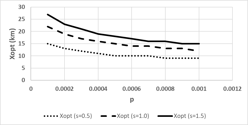
Figure 1 The optimal fire station distance, Xopt=x*, (km), as a function of p, the fire probability per square km and day, and s, the average speed of a fire engine (km/min). Default assumptions: a=10000 (USD), b=0.1, cx=1000 (USD/Day).

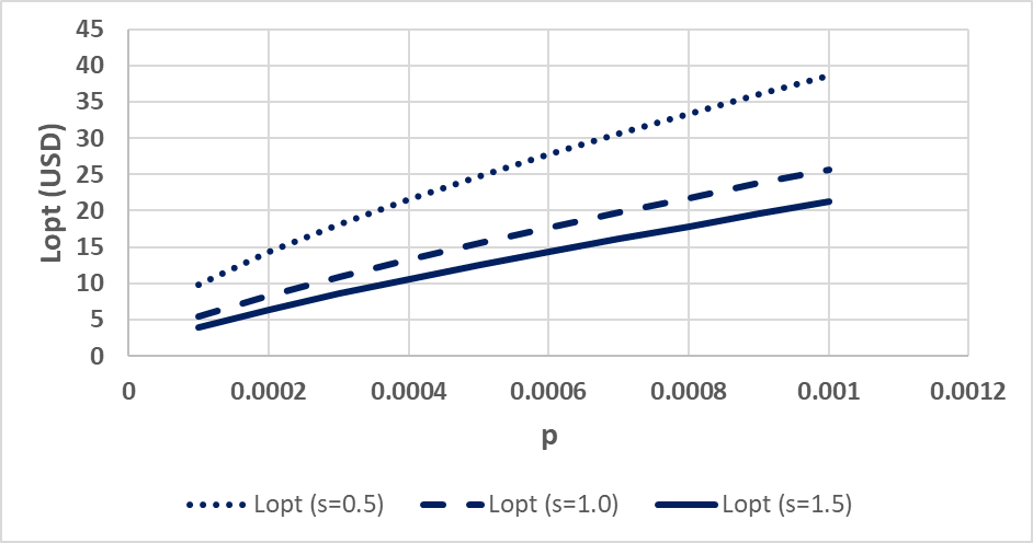
Figure 2 The minimal expected total cost function value, Lopt = L*, (USD), per day and square km, as a function of p, the fire probability per square km and day, and s, the average speed of a fire engine (km/min). Default assumptions: a=10000 (USD), b=0.1, cx=1000 (USD/Day).

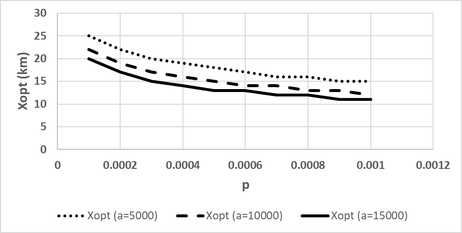
Figure 3 The optimal fire station distance, Xopt=x*(km), as a function of p, the fire probability per square km and day, and a, the expected cost per fire in case the travel time of the fire engines would be zero. Default assumptions: b=0.1, s=1 (km/min), cx=1000 (USD/Day).

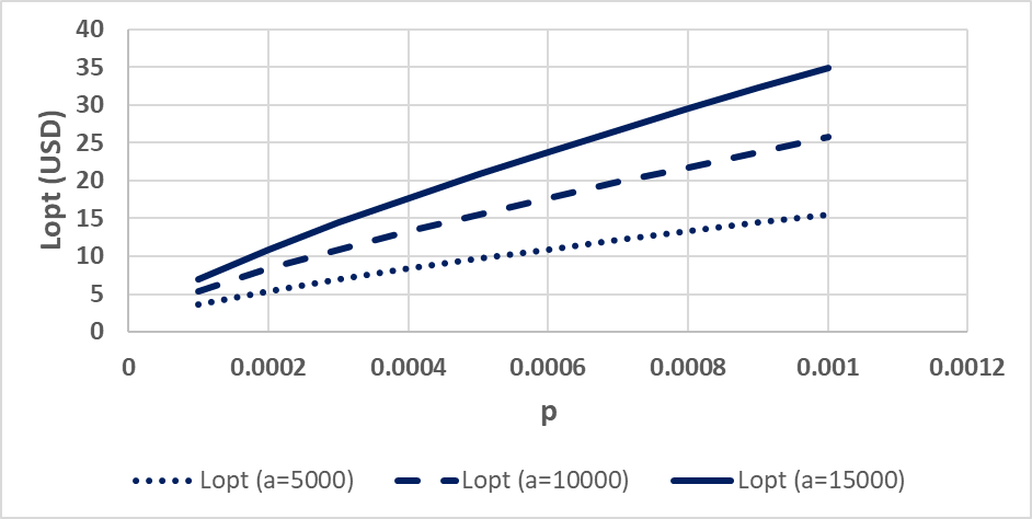
Figure 4 The minimal expected total cost function value, Lopt = L*, (USD), per day and square km, as a function of p, the fire probability per square km and day, and a, the expected cost per fire in case the travel time of the fire engines would be zero. Default assumptions: b=0.1, s=1 (km/min), cx=1000 (USD/Day).

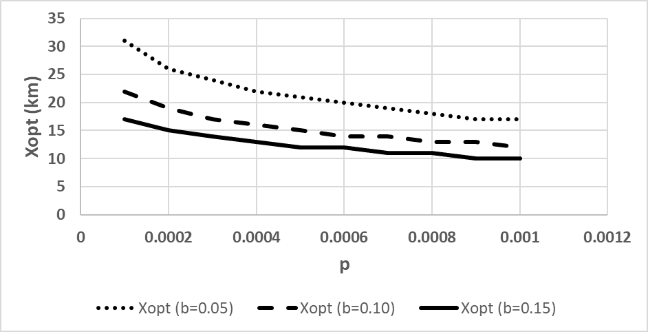
Figure 5 The optimal fire station distance, Xopt=x*, (km), as a function of p, the fire probability per square km and day, and b, the coefficient of exponential growth in the cost function. Default assumptions: a=10000 (USD), s=1 (km/min), cx=1000 (USD/Day).

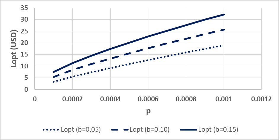
Figure 6 The minimal expected total cost function value, Lopt = L*, (USD), per day and square km, as a function of p, the fire probability per square km and day, and b, the coefficient of exponential growth in the cost function. Default assumptions: a=10000 (USD), s=1 (km/min), cx=1000 (USD/Day).

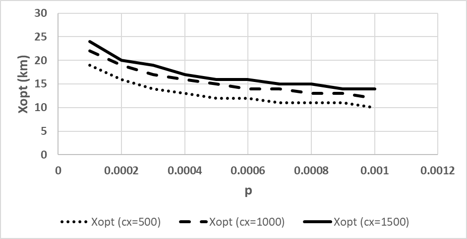
Figure 7 The optimal fire station distance, Xopt=x*, (km), as a function of p, the fire probability per square km and day, and cx, the cost per fire station (USD/day). Default assumptions: a=10000 (USD), b=0.1, s=1 (km/min).

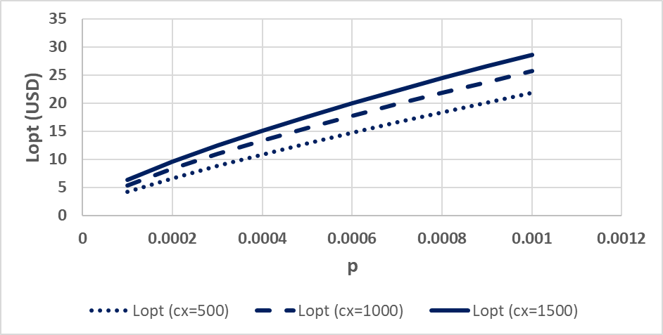
Figure 8 The minimal expected total cost function value, Lopt = L*, (USD), per day and square km, as a function of p, the fire probability per square km and day, and cx, the cost per fire station (USD/day). Default assumptions: a=10000 (USD), b=0.1, s=1 (km/min).

Most countries and periods are different with respect to many things that influence optimal fire management. For this reason, it is important to rapidly adapt fire management, in particular the locations of fire engine companies and the density of the fire defense, to relevant and frequently changing conditions. Purnomo et al.,¹¹ study the forest fire management and conditions in Indonesia. They describe severe problems with large bureaucratic systems and slow decision processes. The authors ask for faster and more efficient fire response. In this paper, we have seen how the optimal density of fire engine companies is affected by changing conditions of different types. Clearly, since temperature, humidity and wind conditions can change considerably and rapidly over time, it is necessary, as Purnomo et al.,¹¹ write, to be able to respond efficiently, with as little delay as possible. The new results and functions have been presented in rather general form. When the approach is applied, however, it is important to explicitly include the relevant facts. For instance, the fire cost function may include costs of firefighting, costs of destroyed forest areas or other property and also costs of emitted CO₂ from the fire. Perhaps, also, in the case of burning forests, one part of the cost may be that the destroyed forest, in the future, will absorb less CO₂ than a forest that did not burn. It is important also to be aware of the differences between fire management strategies in forest regions and in cities. In New York City, for instance, fires can be expected to start and to spread during most times of the year. Even if we have winter conditions, fires can start and grow in buildings. In a forest region, on the other hand, the probability that a fire starts and spreads can be almost zero during rainy periods, and during the long winter season, when everything is covered by deep snow. Travel speed, is as we have seen in this paper, a key parameter when the optimal distances between fire engine companies should be decided. In a city, the travel speed is not severely affected by changing seasons. Of course, sometimes, the traffic and road conditions may be worse than normal. There may be some snow on the roads in the winter, and so on. But mostly, the travel speed is almost constant. Then, fire engine travel times calculated by Kolesar⁶ and Kolesar et al.,⁷ can be used. In forest regions, on the other hand, some roads cannot be used at all during rainy periods.

Furthermore, during the winter, all roads may be covered by snow. Then, the travel times are quite different from what they are during a dry summer period. This dramatically changes the optimal distances between fire engine companies. For these reasons, it is usually rational to keep the density and locations of fire engine companies in cities more or less constant during the year. Then, studies of the type Kolesar et al.⁸ can be useful to guide the permanent positioning of these resources. In sparsely populated forest regions, on the other hand, periodically changing locations are typically optimal. Then, the methods presented in this paper may be useful. Below, some typical examples will be illustrated. The parameters in the cost function can easily be used to describe several things.

Example 1: Assume that the volume of wood per hectare is equal in different places. In a region close to large markets, the value of timber is usually higher than far away from the markets, since the cost of transportation is very different. Hence, the cost of a forest fire per cubic meter of timber is usually higher close to the markets. In the optimization, this is easily taken care of via the parameter a. As a result, the optimal distance between fire stations is larger far from the markets than close to the markets.

Example 2: If the wind speed increases, the fire size and the cost of the fire, increase more rapidly. This can be taken care of via parameter b in the exponential fire cost function. If the wind speed increases, then b increases. As a result, the distance between fire stations should decrease.

Example 3: Assume that it becomes more important than before, to reduce the CO₂ emissions. Then, the cost of fires increases. If you increase parameter a, you will capture this effect. As a result, the optimal distance between fire stations decreases.

Example 4: You may also optimize the properties of the fire engines and the quality of the roads. These factors influence s, the speed of the fire engines, which is a parameter in the optimization problem in this paper. In such an analysis, you would have to expand the optimization model in this article with new decision variables and associated cost functions, representing investments in fire engine capacity and road quality.

The reader is encouraged to define new and expanded decision problems where the present analysis tool is integrated as one component. The list of possible studies is almost unlimited.

It is proved that the optimal distance between fire brigade unit positions, OFD, which minimizes the total expected cost, is unique. (In the analysis, OFD was denoted by x^* in order to make the exposition easier to follow.) OFD is a continuous variable and optimal solutions are usually not integers. The optimal solution can however not be expressed via an explicit function. Then, the OFDs were replaced by integers, OFDIs, for different parameter assumptions. The method enumeration in combination with the fact that the continuous objective function is proved to be strictly convex, makes sure that the optimal integer solutions are found. In this process, also the optimal expected total costs, were derived. With comparative statics analysis, it was proved that the OFD is a strictly decreasing function of the expected number of fires per area unit, a strictly increasing function of the speed of the fire engines, a strictly decreasing function of the parameters of the exponential fire cost function, and a strictly increasing function of the cost per fire station. These effects of parameter changes were also illustrated via graphs in the numerical section. They show how the OFDIs are affected by changes of the different parameters.

None.

The author declares that there is no conflict of interest.

None.

1. Williams AP, Abatzoglou JT, Gershunov A, et al. Observed impacts of anthropogenic climate change on wildfire in California. Earth's Future. 2019;7(8):892–910. 
2. Mohammadi Z, Lohmander P, Kaspar J, et al. The effect of climate factors on the size of forest wildfres (case study: Prague‑East district, Czech Republic). Journal of Forestry Research. 2021.
3. Lohmander P. Dynamics and control of the CO2 level viaa differential equation and alternative global emissions strategies. Int Rob Auto J. 2020;6(1):7–15.
4. Lohmander P. Forest fire expansion under global warming conditions:multivariate estimation, function properties and predictions for 29 countries. Cent Asian J Environ Sci Tech Innov. 2020;1(5):134–142. .
5. Lohmander P. Optimization of forestry, infrastructure and fire management. Caspian J Environ Sci. 2021;19(2):287–316.
6. Kolesar P. A model for predicting average fire company travel times. New York, NY: RAND Institute. 1975.
7. Kolesar P, Walker W, Hausner J. Determining the relation between fore engine travel times and travel distance in New York city. Operations Research. 1975;23(4):614–627.
8. Kolesar P, Blum EH. Square Root laws for fire engine response distances. New York, NY: RAND Institute. 1973.
9. Suzuki T, Satoh E. An analysis on the optimum location of fire department based on ambulance dispatch situation—a case study in Utsunomiya City. Japan Architectural Review. 2020,3(2):241–255.
10. Lohmander P. Adaptive mobile firefighting resources, stochastic dynamic optimizationof international cooperation. Int Rob Auto J. 2020;6(4):150–155.
11. Purnomo EP, Ramdani R, Agustiyara, et al. Bureaucratic inertia in dealing with annual forest fires in Indonesia. Int J Wildland Fire. 2021;30(10):733–744.