New methodology of stable, high accuracy estimation and optimization of stimulated reservoir volume (SRV) forecast is presented in this paper. It includes time-related data segmentation, new multilevel feature engineering, analysis of associations and importance of engineered variables. Among first-level feature engineered variables are three quantile-type variables qRangeDepth, qRangeNorth, and qRangeEast. hese three quantile-type variables are used for SRV estimation. In addition to quantile-type variables, two first level variables -trange and event minute are constructed as the first -level variables. These two variables give compact characterization of distribution of microseismic events in time and are used as predictor variables in ML SRV forecast. Second and third level engineered variables are built via transformation of variables of the first level. Although in this paper we focus on the SRV forecast, the same ideas are applicable to the characterization and forecasting of the plume volume in carbon storage and monitoring applications.

A linear regression method and two ML methods - random forest, and regression tree are used for the SRV forecast. It is demonstrated that in the case of selection of appropriate set of first and second level predictor variables even simplistic linear regression may produce accurate SRV forecasts. Still, machine learning methods produce more accurate forecasts characterized by high values of accuracy parameters r.squared and correlation between SRV and its forecast values. Our results can have a significant impact on the proper design of a hydraulic fracturing operation. It can also be used for monitoring CO₂ plume in carbon sequestration sites.

Keywords: hydraulic fracturing; stimulated reservoir volume (SRV) machine learning; forecast; feature engineering; segmentation; variable importance; stability; carbon sequestration

Microseismic data monitoring is actively developing area of research with its own successes and problems.^1,2 Important parameter that may be derived from microseismic events is stimulated reservoir volume (SRV).^3–7 This parameter is widely used for analysis of well performance and stimulation effectiveness in unconventional reservoirs. Stability of SRV estimation and accuracy of machine learning SRV forecast are directly related to the structure of a set of microseismic events and to parameters derived via events structure analysis. In this paper stable SRV estimation and enhancement of SRV forecast accuracy is achieved via time related segmentation of a set of microseismic events and using feature engineering,^8,9 followed by machine learning forecast. In this paper we use three machine learning methods combined with feature engineering and stochastic simulation of perturbated predictor variables. These methods are widely used in research devoted to environmental science, earth science, and petroleum engineering [17-25]. A new version of feature engineering, named multilevel feature engineering is introduced and used for construction of predictor variables. Randomized Monte Carlo cross validation¹⁰ is used in this paper as the tool for analysis of associations between SRV and constructed predictor variables and analysis of ML forecasts accuracy. Predictor variables used in ML forecasts were built using microseismic data available in the 3D HFTS dataset named "SUGG-A-171 5SM”. This dataset is available at EDX website (https://edx.netl.doe.gov/). Also, see the work of¹¹ on alternative machine learning based approach to predict SRV. More details on machine learning techniques used can be found at Aminzadeh, et al,.¹² Also see Aminzadeh,¹³ and Aminzadeh¹⁴ on reservoir characterization and hydraulic fracturing.

Time-windowed segmentation of microseismic data

Time-windowed segmentation of microseismic data that can also be referred to as 4D Microseismic data is the first step in used in this paper procedure of SRV analysis and SRV forecast. To perform time-related segmentation the microseismic data are presented as a set of records of the following form:

$Record\left(k\right): \left(time\left(k\right), East\left(k\right), North\left(k\right), Depth\left(k\right), magnitude\left(k\right) \right)$   (1)

In Eq. 1 k is index of the record, $1\le k\le kmax$ ; East, North, and Depth are spatial coordinates of the event, magnitude is the recorded magnitude of microseismic events. Each segment contains a 3D subset of records with indexes k(p) defined by Eqs. 2 and 3.

$segmShift*\left(p-1\right)<k\left(p\right)\le segmShift*\left(p-1\right)+Nrec$   (2)

$1\le k\left(p\right)\le Nrec$   (3)

Where Nrec is the number of records in each individual segment, p is index of the segment, segmShift is the time shift between two neighboring segments. To get most stable results, parameter is selected to be much larger compared to segmShift, so that neighbor segments strongly overlap. Results presented in this paper are obtained using parameters segmShift and Nrec defined by Eq. 4.

$SegmShift=2; Nrec=40$   (4)

Feature engineered variables of the first and level

Microseismic events in each segment are characterized by several parameters. Among them are index of the segment p, index of event k, time of event t(k)three spatial parameters North, East and Depth, and magnitude of event. These parameters are used for construction of new variables. Among them are three quantile ranges of spatial coordinates defined by Eqs. 5, 6, and 7.

$yqRangeEast\left(p\right)=quantile(East\left(k\left(p\right),qP=0.995\right)-quantile(East\left(k\left(p\right),qP=0.005\right)$   (5)

$qRangeNorth\left(p\right)=qantile(Nofrth\left(k\left(p\right),qP=0.995\right)-quantile(North(k\left(p\right),qP=0.005)$   (6)

$qRangeDepth\left(p\right)=qantile(Depth\left(k\left(p\right),qP=0.995\right)-quantile(Depthth(k\left(p\right),qP=0.005$   (7)

Four segmented quantiles of time dependent magnitude of microseismic events are defined by Eqs. 8 to 11.

$qMagn1\left(p,\right)=quantile\left(Magnitude\left(p,k\right), qP=0.25\right)$   (8)

$qMagn2\left(p,\right)=quantile\left(Magnitude\left(p,k\right), qP=0.5\right)$   (9)

$qMagn3\left(p,\right)=quantile\left(Magnitude\left(p,k\right), qP=0.75\right)$   (10)

$qMagn4\left(p,\right)=quantile\left(magnitude\left(p,k\right),qP=0.99\right)$   (11)

In Eqs. 5 to 11 $qP$ is quantile probability. Additional first-level variables named trange(p) and eventminute(p) are defined by Eqs. 12 and 13.

$trange\left(k,p\right) =max\left(t\left(k,p\right)\right)-min\left(t\left(k.p\right)\right)$   (12)

$eventminute\left(k,p\right)=60*Nrec/trange\left(k,p\right)$   (13)

In Eqs. 12 and 13 t(k,p) is recorded time of microseismic event with index k in the segment with index p. Quantile probabilities in Eqs. 5, 6, and 7 are equal 0.995 and 0.005. Therefore, only a small number of microseismic events are treated as outliers located outside parallelepiped that defines SRV. Time value assigned to the segment with index p is defined as the first level feature engineered parameter defined by Eq. 14

$Time\left(p\right)=mean(time\left(k\left(p\right)\right)$   (14)

Where time(k(p)) is the time of microseismic event with index k within the segment with index p. Plot of variable Time(p) is shown at Figure 1.

According to Figure 1 values of variable $Time\left(p\right)$ monotonically increase with increase of segment index, although rate of such increase changes with change of segment index. This property of Time (p) variable allows to construct variables trange and eventminute that used in producing SRV forecasts.

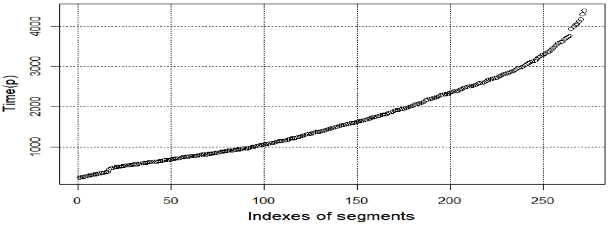
Figure 1 Plot of variable Time (p) with time values assigned to 270 segments.

Variables constructed at the second level of feature engineering.

The following transformation methods are used in feature engineering of the second level variables.

Power-based transformation done according to Eq. 15

$variableT\left(r\right)=abs{\left(variable\right)}^p$   (15)

The Logarithmic transformation defined by Eq. 16.

$variableT=log\left(variable\right)$   (16)

Variables designed according to Eqs 16 and 17 are used as predictor variables in ML forecasts reviewed in this paper. Three additional variables of the second level are defined by Eqs. 17, 18, and 19.

$qrEastNorth =qRrangeEast*qRangeNorth$   (17)

$qrDepthNorth =qRangeDepth*qRangeNorth$   (18)

$qrDepthEast =qRangeDepth*qRangeEast$   (19)

Power-based transformation of normalized variables is done according to Eq. 21.

$variableT\left(r\right)=abs{\left(variable/mean\left(variable\right)\right)}^p$   (20)

Specific form of second level engineered variable is defined as product of several features constructed at the first level. This type of variable is used for SRV calculation. SRV is defined as the volume of orthogonal 3D parallelepiped and is calculated according to Eq. 21.

$SRV\left(p\right)= qRangeEast\left(p\right)* qRangeNorth\left(p\right)* qRangeDepth \left(p\right)$   (21)

Compact description of multilevel feature engineering procedure is presented at Figure 2.

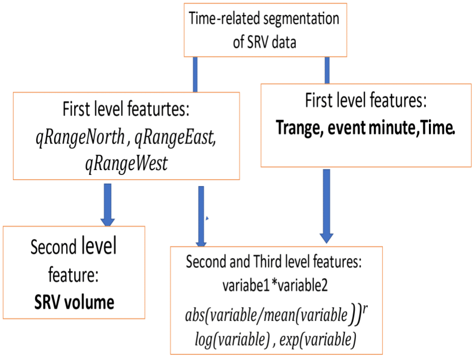
Figure 2 Compact description of multilevel feature engineering.

Analysis of stability of SRV estimation

SRV is calculated in this paper as a function of three feature engineered variables of the first level. Generally, there is no relationship between stability of variables and stability of their function. The goal of this section is to illustrate methodology of analysis of relationships between stability of three variables that define SRV values and their function - SRV and to illustrate that relative stability of calculated SRV is close to stability of SRV. It5 is necessary to note that the more complex problem of stability analysis of SRV forecast is not reviewed in this paper and will be analysed in future research.

Method of stochastic simulation of random noise^15–18 is used in this paper to analyze stability of SRV estimation. The first step in estimation of SRV stability is random perturbation of values of quantile-type variables that characterize spatial distribution of microseismic events. Perturbed versions of three quantile-type variables are calculated according to Eqs 22, 23, and 24.

$RqRangeNorth\left(p,k,n\right)=qRangeNorth+noise\left(p,k,n\right)$   (22)

$RqRangeEast\left(p,k,n\right)=qRangeEast+noise\left(p,k,n\right)$   (23)

$RqRangeDepth\left(p,k,n\right)=qRangeNorth+ noise(p,k,n)$   (24)

Perturbed values of SRV are calculated according to Eq. 25.

$rSVR\left(p,k,n\right)=RqRangeNorth\left(p,kn\right)*RqRangeEast\left(p,k,n\right)*RqRangrNorth\left(p,k,n\right)$   (25)

In Eqs 22-25 n is the index of the perturbation. It is the same in all four equations 22-24, whereas noise components are all different and generated independently from each other. All noise components in Eqs 22-24 are built as uniformly distributed random values with zero mathematical expectation and range of values defined by Eqs 26 and 27.

$-DSRV<noise<DSRV$   (26)

Where

$DSRV=\left(max\left(SRV\right)-min\left(SRV\right)\right)*0.$   (27)

Using parameter DSRV allows to define noise level as fracture of the width of SRV range. Stability of analyzed variables is characterized in this paper by the values of parameter named St. It is defined by Eq. 28.

$St\left(variable\right)=mean\left(variable\right)/\left(mean\left(variable\right)+std\left(variable\right)\right)$   (28)

Where mean(variable) and std(variable) are estimates of mean and standard deviations of analyzed variables calculated using multiple perturbed versions of the same variable.

Forty perturbed SRV versions are shown in Figure 3. According to this figure all forty SRV perturbed versions are very close to each other. Therefore, SRV stability is high.

Figure 3 Plots of 40 perturbed SRV versions.

High stability of SRV estimates is confirmed by results presented in Table. Table 1 and Table 2 show values of association criterion as function of two versions of transformations – simplistic (not normalized and not scaled) and transformed according to Eq. 20. In Table 1 m is index of the version of parameter $Association.$  One can observe that different versions of this parameter are slightly deferent.

According to Table 2, the value of stability parameter that characterizes SRV is slightly smaller than stability values of three spatial variables, but it is still as large as 0.951. Values of stability presented in Table 6 depend on the noise level. Therefore, the information presented in this Table is not sufficient for SRV stability characterization. More informative parameter that characterizes SRV stability is presented in Table 3. This Table contains normalized values of relative stability variable, $relSt,$  This parameter is defined by Eq. 29.

$relSt=3*St\left(Var\right)/(st\left(qRangeEast\right)+St\left(qRangeNorth\right)+St\left(qRangeDepth\right)$   (29)

According to Table 3 relative stability of SRV is about 6% smaller compared to smallest stability of quantile type variables, but it is still as large as 0.979.

Monte Carlo association between SRV and newly constructed variables

In this paper, two criteria are used for selection of the most appropriate predictor variables. The first one is Monte Carlo Association criterion that is used as a tool for preliminary analysis of variables importance. The higher is Monte Carlo association the more important variable is. The second criteria is to use alternative machine learning techniques, including: Linear regression, Random Forrest and Regression tree, to determine the respective value of addition of different variables to the set of predictor variables.

Monte Carlo association criterion is calculated using multiple versions of correlation coefficients between SRV values and values of newly designed variables. Each version of correlation coefficient is obtained using a set of values of correlated variables and SRV built using randomized Monte Carlo resampling.

Monte Carlo association criterion is defined by Eq. 30

$Association\left(var\right)=mea{n}_r(cor(SRV\left(r\right),\left(var\left(r\right)\right)$   (30)

In Eq. 30 SRV(r) and var(r) are values of SRV and variable created via r-th randomized Monte Carlo resampling, cor(SRV{r), var(r)) is correlation coefficient calculated using pair SRV{r) and var(r) (Table 4).

According to Table 5 different variables show different patterns of dependence of values of association criterion from changing values of parameter p. It also follows from Table 5 that parameters trange, qRangeDepth, qRangeEast, and qRangeNorth are characterized by high values of association criterion if p=1.

Analysis of differences in variables importance obtained using different machine learning methods

Criterion Importance is the criterion specifically related to analysis of performance of machine learning methods of specific types.¹⁹ In previous section of this paper analysis of association between potential predictor variable and variable to be predicted was done without considering the fact that different variables may be characterized by different levels of importance to different machine learning methods.

Importance of quantile-type untransformed variables characterizing linear regression, random forest, and regression tree are shown in Table 1. This table illustrates differences in importance values calculated using different ML methods. This means that training sets compiled for different ML methods may include different predictor variables.

According to Table 6 different variables are characterized by different values of parameter importance if different forecast methods are to be used. Four quantiles of magnitudes are characterized by very low values of importance in case of linear regression, but values of this parameter are at much larger in case of regression tree. On the other hand, variables qrgEastNorth and qrgDepthNorth are characterized by values of this parameter significantly larger in case of linear regression compared to random forest.

Analysis of accuracy of machine learning forecast using predictor variables constructed using only information about time of occurrence of microseismic events

This section and the following section of this paper illustrate the possibility of using only time of occurrence microseismic events to produce an accurate enough SRV forecast. Special attention is devoted to usage of predictors of this specific type is due to the relative simplicity of collecting data on time of microseismic events and building training set without use of any additional information about magnitude and spatial distribution of events.

Three forecast methods - linear regression, regression tree, and random forest, are used in this chapter, and accuracy of forests done by these methods is analyzed. Regression tree^20–22 is generalization of two methods – linear regression and decision tree. The algorithm of regression tree includes iterative partition of the input data set into smaller subgroups and then fit regression model for each subgroup. This machine learning method has been used in different areas of science, such as geology environmental science, and medical science [-]. Random Forest Regression^23–25 is a supervised learning algorithm that uses ensemble learning method for regression and combines ensemble learning with decision tree algorithm. This method is widely used in different science areas.

Forecasts by all three methods is done according to Eqs 31 and 32 using functions train, $trainControl$ and predict available in opens source CARET package, short for classification and regression training.²⁶

$obj<-train\left(srvk~., varTrainSset, method=met, trainControl=fitConjtrol\right)$   (31)

$pred<-predict\left(obj,varTestSet\right)$   (32)

In Eqs. 31 and 32 $VarTrainset$ and $varTestSet$ are, respectively, sets of predictor variables in train and test sets, met is forecast method taking one of three values - linear regression, regression tree, and random forest.

One of the goals of this and the following section is to do quantitative analysis of accuracy of forecast performed by three forecast methods. Another goal is to illustrate the possibility of using only time of occurrence microseismic events to construct a set of predictor variables using which may lead to accurate enough SRV forecast. Special attention to usage of predictors of this specific type is due to the relative simplicity of collecting data on time of microseismic events and building training set without use of any additional information about magnitude and spatial distribution of events.

Variables of the first and second levels used as predictors in this section are: var1, var2, var3, var4.

These variables are defined by Eqs 33 and 34.

$var1=-trange; var2=eventminute$   (33)

$var3=trang{e}^3 var4=eventminut{e}^3$   (34)

The forecast model is defined by Eq. 33.

$SRV~var1+var2+var3+var4$   (35)

SRV itself and SRV forecasts done by linear regression, random forest, and regression tree are shown Figures 4–6.

According to Figure 4 accuracy of SRV forecast done by linear regression is low. The values of forecast shown at Figure 4 fluctuate strongly and large SRV values are strongly different from respective forecast results.

Figure 5 and Figure 6 show forecasts done by regression tree and random forest. According to these figures accuracies of forecasts done by both regression tree and random forest is high, whereas in case of linear regression forecast accuracy is much lower.

Quantitative characterization of accuracy of forecasts done using forecast shown at Figures 4–6 is presented in Table 7.

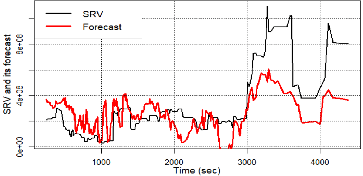
Figure 4 SRV and SRV forecast done using linear regression.

Figure 5 SRV and SRV forecast done using regression tree.

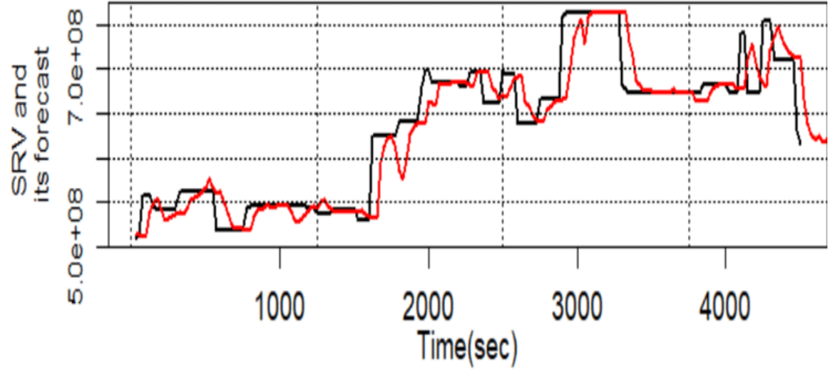
Figure 6 SRV and SRV forecast done using random forest.

According to Table 7 best results are obtained using regression tree, whereas linear regression obviously underperforms.

Improvement of accuracy of SRV forecast using six newly designed predictor variables

This section presents additional illustrations of the importance of feature engineering used as a tool for preparing to machine learning forecast.

Forecast model used in this section is defined by Eq. 36

$SRV~trange+eventminute+var3+var4+var5 +var5+var6$   (36)

Where var4 and var5 are defined by Eqs 35 and 36

$var5==log\left(trange\right)$   (37)

$var6==log\left(eventminute\right)$   (38)

Values of correlation coefficients $cor\left(SRV, Predictor\right)$  are shown in Table 8. According to this table constructed variables var5 and var6 are characterized by absolute values of correlation coefficients exceeding those of initial variables trange and eventminute. Therefore, if the machine learning model defined by Eq. 34 is used, then more accurate forecasts may be produced.

Figure 7 illustrate domination of absolute values of correlation coefficients cor(SRV, Predictor) calculated using predictors var5 and var6. Horizontal discreet line is drawn at the value of correlation coefficient that characterizes variable trange. One can observe that values of correlation coefficients that characterize predictors eventminute, var3, and var4 are3 are below discreet line, whereas correlation coefficients of variables var5 and var6 are3 above this line.

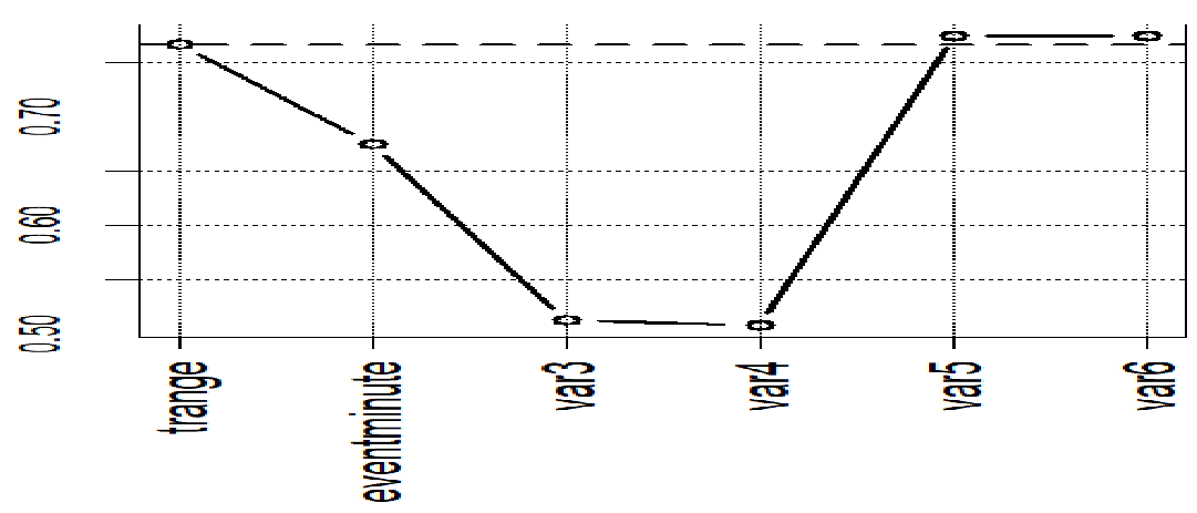
Figure 7 Plot of absolute values of correlation coefficients.

SRV itself and SRV forecasts done by done by linear regression, random forest, and regression tree are shown at Figures 8–10.

Quantitative characterization of accuracy of forecasts done using forecast shown at Figures 8–10 is presented in Table 13.

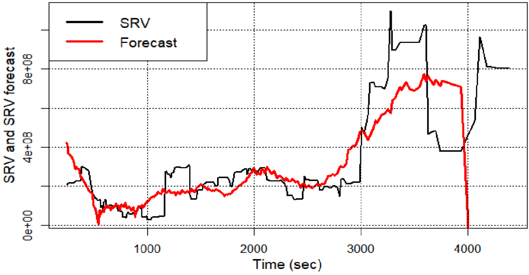
Figure 8 SRV and SRV forecast done using linear regression.

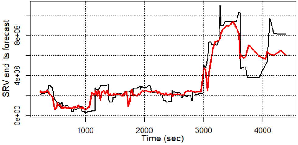
Figure 9 SRV and SRV forecast done using regression tree.

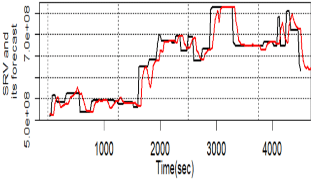
Figure 10 SRV and SRV forecast done using random forest.

According to Table 9 the best results are obtained using regression tree.

1. New procedure of stable, high accuracy SRV estimation and optimization of SRV forecast is presented in this paper. It includes time-related data segmentation, new multilevel feature engineering, analysis of associations and importance of engineered variable and machine learning forecast.
2. Multilevel feature engineering introduced i8nn this paper and utilized in construction of predictor variables of different levels
3. Among time-dependent predictor variables of the first level are variables trange and In addition to these time dependent variables, first-level quantile-type variables qRangeDepth, dRangeEast, and qRangeNorth are constructed.
4. Variables of the second level are built using power and logarithmic transforms of the first level variables. Stimulated reservoir volume (SRV) is calculated as the second level feature engineered variable. It is defined as the product of three first level quantile-type variables – qRangeNorth, qRangeEast, and Using quantile-type variables for SRV calculation allows to exclude effect of outliers.
5. Estimated SRV values are characterized by high stability. Estimated SRV relative stability is only 5% lower than relative stability of quantile-type variables used for SRV
6. Parameters r.squared and mutual correlations between CRV and SRV forecasts are used to quantitively characterize accuracy of SRV forecasts Results of analysis of accuracy of SRV forecasts demonstrate that accuracy of forecast done using even such simplistic method as linear regression is characterized by high accuracy if appropriate set of feature engineered predictor variables is used. Forecasts done by more complex ML methods are characterized by even higher accuracy. For instance, forecast done using machine learning method random forest is characterized by values of accuracy parameters r.squared and correlation between SRV and its forecast equal, respectively, 0.798 and 0.894.

We acknowledge the contribution of Dr. Ali Rezaei for locating the test data and other technical input.

FACT Inc.

The author declares no conflict of interest in writing the manuscript.

1. Xin X, David L. Feature engineering for machine learning and data analytics. Feature engineering for machine learning and data analytics. 335-358. Research Collection School of Information Systems. 2018
2. Andre Elisseeff. An introduction to variable and feature selection. Journal of Machine Learning Research. 2003:1157–1182.
3. Enrico C, David WE, Joshua PJ, et al. Detection and analysis of microseismic events using a Matched Filtering Algorithm (MFA). Geophysical Journal International. 2016;206(1):644–658.
4. Leo E, Michael T, Jessica G. Challenges for microseismic monitoring. SEG Technical Program Expanded Abstracts. 2011.
5. Mario P. GillespieSSA: Implementing the Gillespie Stochastic Simulation Algorithm in R. Journal of Statistical Software. 2008;25(12).
6. Wang W, Zheng D, Sheng G, et al. A review of stimulated reservoir volume characterization for multiple fractured horizontal well in unconventional reservoirs. Advances in Geo-Energy Research & Capillarity. 20171(1).
7. Ren L, Lin R, Zhao J. Stimulated reservoir volume estimation and analysis of hydraulic fracturing in shale gas reservoir. Arab J Sci Eng. 2018;43:6429–6444.
8. Greenwell B. Feature & target engineering. Hands-On Machine Learning with R. Chapman & Hall; 2019:41–75.
9. Alice Z; Amanda C. Feature engineering for machine learning: principles and techniques for data scientists. O'Reilly Media, Inc; 2018.
10. Simon K, Fred A, George C, et al. Rock permeability forecasts using machine learning and monte Carlo committee machines. Journal of Sustainable Energy Engineering. 2018.
11. Rezaei A, Aminzadeh F. A data-driven reduced-order model for estimating the Stimulated Reservoir Volume (SRV). Energies. 2022;15(15):5582.
12. Aminzadeh F, Temizel C, Hajizadeh Y. Artificial intelligence and data analytics for energy exploration and production. 2022. ]
13. Aminzadeh F. Reservoir characterization. John Wiley: Reservoir Characterization, Wiley Online Books; 2021. ISBN 9781119556213.
14. Aminzadeh F. Hydraulic fracturing. John Wiley: Hydraulic Fracturing and Well Stimulation, Wiley Online Books. 2019. ISBN 978111955698.
15. Slepoy A, Thompson AP, Plimpton SJ. A constant-time kinetic Monte Carlo algorithm for simulation of large biochemical reaction networks. J Chem Phys. 2008;128(20).
16. Cai X. Exact stochastic simulation of coupled chemical reactions with delays. J Chem Phys. 2007;126(12).
17. Press WH, Teukolsky SA, Vetterling WT, et al. Section 17.7. Stochastic simulation of chemical reaction networks. Numerical Recipes: The Art of Scientific Computing. 3rd edn. New York: Cambridge University; 2007.
18. Ramaswamy R, Sbalzarini IF. A partial-propensity formulation of the stochastic simulation algorithm for chemical reaction networks with delays" (PDF). J Chem Phys. 2011;134(1).
19. Gevrey M, Dimopoulos I, Lek S. Review and comparison of methods to study the contribution of variables in artificial neural network models. Ecological Modelling. 2003;160(3):249–264.
20. Leathwick JR, Hastie T. Machine learning applied to SRV modeling, fracture characterization, well interference and production forecasting in low permeability reservoirs. Journal of Animal Ecology. 2008;77:802–813.
21. Friedman JH, Meulman JJ. Multiple additive regression trees with application in epidemiology. Stat Med. 2003;22:1365–1381.
22. Loosvelt L, Peters J, Skriver H, et al. Random Forests as a tool for estimating uncertainty at pixel-level in SAR image classification. International Journal of Applied Earth Observation and Geoinformation. 2012;19:173–184.
23. Navada A, Ansari AN, Patil S, et al. Overview of use of decision tree algorithms in machine learning. 2011 IEEE Control and System Graduate Research Colloquium. 2011:37–42.
24. McKay G, Harris JR. Comparison of the data-driven random forests model and a knowledge-driven method for mineral prospectively mapping: a case study for deposits around the Huritz Group and Nueltin Suite, Nunavut, Canada. Natural Resources Research. 2015.
25. Rodriguez-Galiano M, Sanchez-Castillo M, Chica-Olmo M, et al. Machine learning predictive models for mineral prospectivity: An evaluation of neural networks, random forest, regression trees and support vector machines. Ore Geology Reviews. 2015;71:804–818.
26. Kuhn. Building Predictive Models in R Using the caret. 2008.