In the present work, damped free and forced vibrations of single-walled piezoelectric carbon nanotubes under longitudinal magnetic field due to surface effects surrounded on a non-linear viscoelastic medium using the nonlocal Euler-Bernoulli beam theory and multiple time scales method are investigated. Lorentz force equation is used to obtain the vertical force due to the applied voltage to the system. The surface effects as well as a combinational non-linear viscoelastic foundation are considered, and finally, the dynamic equilibrium equations are used, and non-linear equations of motion are extracted. In the following, the Galerkin and multiple time scales methods are used, and finally, analytical solutions are extracted as the non-linear free and forced vibrational responses of the system. The relevant coefficients of the extracted analytical solutions are discovered for two both simple support (S-S) and clamped (C-C) boundary conditions. In the following, , and the effects of the different parameters such as non-local parameter as well as electric-magnetic fields, effect of hardness-linear damping parameters of nonlinear considered viscoelastic foundation, applied magnetic field, base modes for different forms considering surface effects, and etc. will be studied. As one the results of this study, the presence of a non-local parameter has increased the curvature deviation to the right and the stiffening effect. In other words, the non-local parameter is a factor to increase the nonlinear effect of the system. Also, it is predictable that as the load affect position moves away from the center of the single-walled piezoelectric carbon nanotube toward the supports, the amplitude of the dynamic response decreases significantly, and this relative reduction is greater for the C-C boundary condition than for the S-S boundary condition. It is also important to note that the location of the load has no effect on the rate of deviation of the curve peak, and the degree of nonlinearity of the vibrational response of the system.

Keywords: nonlocal euler-bernoulli beam theory, non-linear non-local damped forced vibration, viscoelastic piezoelectric carbon nanotubes, magnetic field, non-linear viscoelastic foundation, surface effects

Having unique physical and chemical properties such as extremely high tensile strength and rigidity, combined with very low density, makes CNTs an essential part of all industrial fields. Nanotubes are critical members of the design and fabrication of nanoelectromechanical systems.¹ Microelectromechanical and nanoelectromechanical systems are the essential applications of piezoelectric generators.² Surface effects are other phenomena that occur due to the static balance of atoms on the surface.³ These effects on elastic bodies are divided into three categories: surface tension, residual surface stress, and surface density.⁴ Indeed, surface effects will play a serious role when the surface-to-volume ratio increases.^5–6 Finally, surface effects may have an important role in the vibration analysis of nanotubes.^7–8

The damped forced vibration of SWCNTs was analyzed using a new shear deformation beam theory.⁹ In this new shear deformation beam theory, there was no need to use any shear correction factor, and also the number of unknown variables was the only one that was similar to the Euler-Bernoulli beam hypothesis. The torque effect of an axial magnetic field on a functionally graded (FG) nano-rod has been studied to capture size effects under magnetic field using Maxwell’s relation.¹⁰ As an important result of this study could be mentioned that an FG nano-rod model based on the nonlocal elasticity theory behaves softer and has a smaller natural frequency. Investigation of free vibration of viscoelastic nanotube under longitudinal magnetic field also was studied in recent years.¹¹ According to a deep investigation on the natural frequencies and effect of different parameters such as the nonlocal parameter, structural damping coefficient, material length scale parameter, and the longitudinal magnetic field, the results of this research may be helpful for understanding the potential applications of nanotubes in Nano-Electromechanical System. Many studies in the literature are focused on the investigation of the vibration analysis of nanostructures in an elastic medium. The vibrational response of a SWCNT member considered in an elastic medium to transport a viscous fluid,¹² Investigating the vibration of a DWCNT embedded in an elastic medium despite initial axial forces,^13,14 Investigating the vibration of nanotubes in conditions where the surrounding medium is considered elastic,¹⁵ investigating the nonlinear free vibration of a DWCNT member considering the von Karman assumption in order to apply nonlinear effects and nonlinear,¹⁶ nonlinear vibration of a DWCNT by C-C boundary condition in an elastic medium using the nonlinear van der Waals forces, and also the von Kármán geometric to consider nonlinearity,¹⁷ Investigating the forced vibration of a DWCNT with the potential to carry a moving nanoparticle,¹⁸ investigation of the nonlinear vibration of an MWCNT in thermal environments,¹⁹ vibration analysis of an MWCNT by thermal effects, and also considering the size effects on the large amplitude,²⁰ studying free vibration of SWCNT with elastic effects for different boundary conditions,²¹ vibration of SWCNT with an elastic medium due thermal conditions,²² thermal-mechanical effects consideration to study vibration and buckling instability of a SWCNT that carry out fluid, and also is rested on an elastic foundation,²³ electro-thermo-mechanical effects consideration to study vibration of boron nitride nanorod that is in elastic medium by non-uniform and non-homogeneous properties,²⁴ buckling analysis of SWCNT on a viscoelastic foundation for different boundary conditions,²⁵ buckling investigation of SWCNT under thermal effects that is in an elastic medium with one elasticity parameter,²⁶ and buckling behavior of single-walled CNT considering thermal effect in an elastic medium²⁷ were studied using non-local theory of elasticity. another theory that can be considered as size-dependent continuum theories, and also can be used to study the electro-thermal transverse vibration of CNT in an elastic medium was presented based on the non-local shell theory as well as piezoelasticity properties of system.²⁸ Continuum shell theory by considering nonlocal effects was used to study free vibration of single-walled carbon nanotubes by non-homogenous elastic medium.²⁹ Using multiple elastic models of beams as well as continuum mechanics theory, non-linear free vibration of multi-walled carbon nanotubes was studied.³⁰ Nonlinear vibration as well as thermal stability and of pre/post buckling due to temperature effects, and also size-dependent FG beams designed on an elastic foundation was studied based on the modified couple stress theory.³¹ The multiple time scales method, as a perturbation method, is known as an efficient technique in nonlinear differential equations analysis. Multiple scale method was used to study free and forced vibration of beams as well as DWCNT on an elastic medium by considering geometric nonlinearity and S-S boundary condition.^32–34 Non-local elasticity theory was used to study tensioned nanobeam nonlinear vibration with considering various boundary conditions.^35,36 The non-local Euler–Bernoulli theory of elasticity³⁷ can be considered as a theory to modify nanoscale as well as nanostructers models that greatly has been used in modelling carbon nanotubes due to the size-effects in nanoscale behavior. Several references in the literatures can be found on the basis of the nonlocal theory of elasticity.^38,39 In some of the recent relevant papers, the nonlinear frequency response of single-walled carbon nanotubes to primary resonance has been studied based on the nonlocal Euler-Bernoulli beam theory.^40–48 The nonlocal Euler–Bernoulli elasticity theory also has been greatly used to study Nonlocal instability of cantilever piezoelectric carbon nanotubes by considering surface effects subjected to axial flow,⁴⁹ Linear free vibration analysis of piezoelectric SWCNTs that the results are extracts considering linear part of a new general nonlinear viscoelastic foundation without considering external force,⁵⁰ Vibration analysis of piezoelectric nanowires with surface and small scale effects,⁵¹ Flexoelectric and surface effects on size-dependent flow-induced vibration and instability analysis of fluid-conveying nanotubes based on flexoelectricity beam model‏,⁵² and Size-dependent nonlinear vibration of functionally graded composite micro-beams reinforced by carbon nanotubes with piezoelectric layers in thermal environments.⁵³ Consequently, due to lots of the presented works in the literature, the objective of the present work is to study damped free and forced vibration of single-walled piezoelectric carbon nanotubes under longitudinal magnetic field considering surface effects resting on a non-linear viscoelastic foundation based on the nonlocal Euler-Bernoulli beam theory as well as multiple time scales and Galerkin methods. A theoretical and numerical study on non-linear nonlocal free and forced vibration responses are performed. This study, considering surface effects, develops a theoretical response for the non-linear nonlocal vibration of piezoelectric carbon nanotubes located on a non-linear viscoelastic foundation, and attenuation factors due to the external magnetic field and piezoelectric voltage Using Galerkin and multiple time scales methods. Surface effects, which harden the surface of nanotubes, are created by the formation of homogeneous masses by Van forces in the waltz. In the following, considering different boundary conditions of the system (S-S and C-C), the relevant coefficients of the developed analytical response are determined. Finally, the vibrational response parameters such as Amplitude-frequency response curves of nonlinear forced vibration, and etc. will be generally investigated for different boundary conditions, and the effects of the different parameters such as non-local parameter and electric-magnetic fields, Effect of hardness-linear damping parameters of viscoelastic foundation, applied magnetic field, base modes for different forms considering surface effects, and etc. will be studied.

Scheme of the considered system

Figure 1 shows structural schematics of a piezoelectric single-walled carbon nanotube with an inner diameter , outer diameter , thickness , length , mass per unit length , and elastic modulus , subjected to voltage and a magnetic field of magnitude . This nanotube, subjected to a harmonic external point load, resting on a nonlinear viscoelastic foundation. Figure 2 shows discrete model of the single walled carbon nanotube by coordinate system.

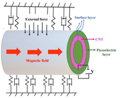
Figure 1 Scheme of the single-walled piezoelectric carbon nanotubes under longitudinal magnetic field subjected to voltage and resting on nonlinear viscoelastic foundation with surface layer.

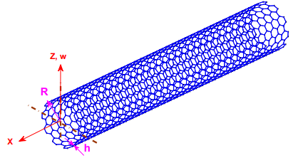
Figure 2 Scheme of the discrete model of the single walled carbon nanotube by coordinate system.

Non-local effects

Generally, nanoscale or microstructure analysis methods can be classified into three categories: molecular simulation, non-classical continuous environment, and multi-scale.⁵⁴ The molecular simulation methods, which simulated atoms and their bonds, investigate nanostructures' behavior more profound than other methods. The high computational volume of this method makes it possible to simulate only small nanostructured dimensions using this method.^55,56 Molecular methods are divided into quantum mechanics, molecular dynamics, and molecular mechanics.⁵⁷ Complex energy functions are used to explain the motion of elementary particles in quantum mechanics. However, this method is associated with computational limitations due to the complexity of the equations used. In the molecular dynamics method, the motion of atoms is studied concerning their adjacent bonds. Atoms are known as rigid particles that are affected by the potential field of neighbouring atoms. The last one, the molecular mechanical method, is based on the displacement of interatomic bonds with beam and spring elements. Potential energy can express the field of interatomic forces in atomic structures. Equalizing the beam and spring elements' potential energy and strain energy, the mechanical properties are obtained equally. In classical theory, the stress state at a particular point can be calculated if the strain state is known at that point. Whereas, in non-classical theory, such as non-local tension theory, the strain state must be known throughout the range to obtain the stress state at a particular point. All other proposed theories based on non-classical continuum mechanics, including strain gradients and coupled stress theories, relate to two-dimensional elasticity.^58–60 Therefore, nonlocal stress tensor can written as follows:^61,62

$\sigma \left(X\right)=\underset{V}{\overset{}{{\displaystyle \int }}}k\left(\left|X^{\prime }-X\right|, \tau \right)T\left(X^{\prime }\right)dV$   (1)

$T\left(X\right)=C\left(X\right):\epsilon \left(X\right)$   (2)

That $\sigma \left(X\right)$ is nonlocal stress tensor at point $X$ , $\left(\left|X^{\prime }-X\right|, \tau \right)$  is nonlocal modulus, is a material constant, $T\left(X\right)$ is classical stress tensor, is $\epsilon \left(X\right)$ strain tensor and $C\left(X\right)$ is elasticity tensor. Because of that solving of the integral constitutive Equation (1) is complicated, a simplified differential for is greatly used as follows:

$T=\left(1-\mu {\nabla }^2\right)\sigma , \mu ={\tau }^2{l}^2$   (3)

Where $\mu$ is non-local coefficient and is ${\nabla }^2$  Laplacian operator. Also, $\tau$ and $l$ are material constant.⁶¹ Finally, nonlocal stress tensor for a beam must satisfy equation (4):

$\sigma \left(X\right)-{\left(\tau l\right)}^2\frac{{\partial }^2\sigma \left(X\right)}{\partial X^2}=E\epsilon \left(X\right)$   (4)

Where is a constant that known as the classical elasticity modulus.

Now, using the existing stress relations in the non-local theory, the relationship between the local bending torque $M^l\left(x,t\right)$  and the non-local torque $M^{nl}\left(x,t\right)$  at the cross section of the nanotube is written as follows⁶³:

$\left(1-{\left(\tau l\right)}^2\frac{{\partial }^2}{\partial x^2}\right)M^{nl}\left(x,t\right)=M^l\left(x,t\right)$   (5)

In equation (5), $\text{μ }$ is the parameter of the nanotube size scale, which is also known as the non-local parameter.

Assume $\overrightarrow{U}=\left(u,v,w\right)$  as the displacement field of the nanostructure; the Lorentz force $f_l$  is equal to⁶⁴:

$\overrightarrow{f_l}=\eta \left(\overrightarrow{J}\times \overrightarrow{H}\right)$   (6)

Where J stands for the current density and H is the magnetic field strength vector in the environment. Also, in equation (6):

$\overrightarrow{J}=\nabla \times \overrightarrow{h}$   (7)

That:

$\overrightarrow{h}=\nabla \times \left(\overrightarrow{U}\times \overrightarrow{H}\right)$   (8)

Therefore, by considering longitudinal magnetic field:

$\overrightarrow{h}=-H_x\left(\frac{\partial v}{\partial y}+\frac{\partial w}{\partial z}\right)\overrightarrow{i}+H_x\frac{\partial v}{\partial x}\overrightarrow{j}+H_x\frac{\partial w}{\partial x}\overrightarrow{k}$  (9)

$\overrightarrow{J}=H_x\left(-\frac{{\partial }^{2}v}{\partial x\partial z}+\frac{{\partial }^{2}w}{\partial x\partial y}\right)\overrightarrow{i}-H_x\left(\frac{{\partial }^{2}v}{\partial y\partial z}+\frac{{\partial }^{2}w}{\partial x^2}+\frac{{\partial }^{2}w}{\partial z^2}\right)\overrightarrow{j}+H_x\left(\frac{{\partial }^{2}v}{\partial x^2}+\frac{{\partial }^{2}v}{\partial y^2}+\frac{{\partial }^{2}w}{\partial y\partial z}\right)$   (10)

Finally, the Lorentz force is:

$\overrightarrow{f_l}=f_x\overrightarrow{i}+f_y\overrightarrow{j}+f_z\overrightarrow{k}=\eta \left[0\overrightarrow{i}+H_x{}^2\left(\frac{{\partial }^{2}v}{\partial x^2}+\frac{{\partial }^{2}v}{\partial y^2}+\frac{{\partial }^{2}w}{\partial y\partial z}\right)\overrightarrow{j}+H_x{}^2\left(\frac{{\partial }^{2}w}{\partial x^2}+\frac{{\partial }^{2}w}{\partial y^2}+\frac{{\partial }^{2}v}{\partial y\partial z}\right)\right]$   (11)

Therefore, along the $x,y,z$ directions:

$f_x=0$

$f_y=H_x{}^2\left(\frac{{\partial }^{2}v}{\partial x^2}+\frac{{\partial }^{2}v}{\partial y^2}+\frac{{\partial }^{2}w}{\partial y\partial z}\right)$

$f_z=H_x{}^2\left(\frac{{\partial }^{2}w}{\partial x^2}+\frac{{\partial }^{2}w}{\partial y^2}+\frac{{\partial }^{2}v}{\partial y\partial z}\right),$   (12)

Therefore, considering $w\left(x,y,z,t\right)=w\left(x,t\right)$ , the vertical force affecting the lateral vibration per unit length of the Euler-Bernoulli nanotube is according to the following equation:

$F_{lz}=\underset{A}{\overset{}{{\displaystyle \int }}}{f}_{z}dA=\left(\eta A H_x{}^2\right)\frac{{\partial }^{2}w}{\partial x^2}$   (13)

In this study, vibration analysis of SWCNTs embedded in viscoelastic medium is presented. In this case, it is assumed that the chemical bonds of SWCNT to be formed generally between the external surface of the carbon nanotube and the viscoelastic medium (see Figures 1 and 2). In this study, the present viscoelastic foundation has linear Winkler stiffness, nonlinear stiffness, linear viscosity damping, and the attenuation is nonlinear. Therefore, in the present work, the force coming from the nonlinear viscoelastic medium could be considered in the general form as follows:

$F_{medium}=F_{linear}+F_{nonlinear}=$

$\left(F_{linea{r}_k}+F_{nonlinea{r}_k}\right)+\left(F_{linea{r}_c}+F_{nonlinea{r}_c}\right)=$

$\left[\left(k_{1}w\left(x,t\right)+(k_3{w}^3\left(x,t\right)\right)\right]+\left(c_0+c_2{w}^2\left(x,t\right)\right)\frac{\partial w\left(x,t\right)}{\partial t}),$   (14)

That includes spring element $k_1$ , nonlinear spring $k_3$ , linear damper $c_0$ , and nonlinear damper $c_2$ .

One of the characteristics that distinguish nanomaterials is their surface effects. There are two essential and mechanically distinct surface effects in nanostructures: surface stress and surface elasticity. Atoms on the surface have different bonds than atoms in the balk, and surface stresses lead to these atoms being at the minimum energy level. Also, in nanostructures, surface elasticity occurs due to the lack of bonded neighbors in surface atoms.^65,66

According to Euler-Bernoulli beam theory, the axial and transverse displacement fields can be considered as follows:

$u(x,y,z,t)=U^0-z\frac{\partial w}{\partial x}$

$w\left(x,y,z,t\right)=w\left(x,t\right),$   (15)

Therefore, the only nonzero (axial) strain of this beam at any point is expressed by the following equation:

${ϵ}_{\text{xx}}=\frac{\partial {\text{U}}^0}{\partial \text{x}}-\text{z}\frac{{\partial }^2\text{w}\left(\text{x},\text{t}\right)}{\partial {\text{x}}^2}$   (16)

Where ${ϵ}_0$  is the axial strain applied to the structure and $\text{w }\left(\text{x},\text{ t}\right)$ is also the transverse displacement (bending) at the desired location x on the center plate of the nanotube. Let's suppose ${\text{E}}_{\text{z}}$  is the electric field created by the electric potential $\Phi$ assuming that this field exists only in the direction of the z-axis where Z indicates the distance from the center of the arrow, then the relationship between the electric current created and the existing electric potential is:⁶⁷

${\text{E}}_{\text{z}}=-\frac{\partial \Phi }{\partial \text{z}}$   (17)

For the surface piezoelectric model, the surface-related structural relationships are different from the bulk volume equations. If the direction of polarization of the piezoelectric medium is assumed in the direction of the z-axis, the stress-strain structural equations related to the surface of the piezoelectric carbon nanotube-based on the relationships presented are written as follows:^3–5

${\sigma }_{\text{x}}^{\text{s}}={\sigma }_{\text{x}}^0+{\text{c}}_{11}^{\text{s}}{\in }_{\text{x}}-{\text{e}}_{31}^{\text{s}}{\text{E}}_{\text{z}}$   (18)

${\text{D}}_{\text{x}}^{\text{s}}={\text{D}}_{\text{x}}^0$   (19)

In equations (18) and (19), ${\sigma }_{\text{x}}^{\text{s}}$  and ${\text{D}}_{\text{x}}^{\text{s}}$  are axial surface stress and electric surface displacement, respectively. The parameters ${\sigma }_{\text{x}}^0$ , ${\text{D}}_{\text{x}}^0$ , ${\text{e}}_{31}^{\text{s}}$  and ${\text{c}}_{11}^{\text{s}}$  indicate the residual surface stress, the residual electrical displacement, the surface piezoelectric constant, and the elastic surface constant, respectively. On the other hand, in piezoelectric carbon nanotubes, the structural relationship between bulk stress and bulk strain would be obtained as follows:⁶⁸

${\sigma }_x=C_{11}{\in }_x- e_{31} E_z$

${\text{σ}}_{\text{x}}\text{=} {\text{C}}_{\text{11}}{\in }_{\text{x}}- {\text{e}}_{\text{31}} {\text{E}}_{\text{z}}$   (20)

${\text{D}}_{\text{z}}={\text{e}}_{31}{ϵ}_{\text{x}}+{\text{k}}_{33}{\text{E}}_{\text{z}}$   (21)

That ${\sigma }_x$   ${\text{σ}}_{\text{x}}$  and ${\text{D}}_{\text{z}}$ represent the classical stress tensor component and the electrical displacement, respectively. Also, ${\text{C}}_{11}$ , ${\text{e}}_{31}$ , and ${\text{k}}_{33}$  are the elastic constant, piezoelectric constant, and dielectric constant of nanotubes, respectively.

In the absence of free electric charge $\frac{\partial {\text{D}}_{\text{z}}}{\partial \text{z}}=0$ , and the potential energy boundary conditions related to the voltage applied to the external environment of the nanotube is obtained from the following equation:

$\Phi (\frac{\text{D}}{\text{2}})=V, \Phi (-D/2) = 0$   (22)

By placing the relation (16) in equation (18), and then placing them in the constitutive equations (20) and (21) as well as using Gauss's law, the axial stress equations (in the local area) on the surface and volume of bulk nanotubes in the local space will be written as follows:

${\sigma }_{\text{x}}={\text{C}}_{11}{ϵ}_0-{\text{e}}_{31}\frac{\text{V}}{\text{D}}-\left({\text{C}}_{11}+\frac{{\text{ e}}_{31}{}^2}{{\text{k}}_{33}}\right)\text{z }\frac{{\partial }^2\text{w}\left(\text{x},\text{t}\right)}{\partial {\text{x}}^2}$   (23)

${\sigma }_{\text{x}}^{\text{s}}={\sigma }_{\text{x}}^0+{\text{c}}_{11}^{\text{s}}{\in }_{\text{0}}- {\text{e}}_{31}^{\text{s}}\frac{\text{V}}{\text{D}}-\left({\text{C}}_{11}^{\text{s}}+\frac{{\text{e}}_{31}^{\text{s}}{\text{ e}}_{31}}{{\text{k}}_{33}}\right)\text{z }\frac{{\partial }^2\text{w}\left(\text{x},\text{t}\right)}{\partial {\text{x}}^2}$   (24)

The equations of motion for the considered SWCNT, as shown in Figure 1, can be extracted as follows:

$[\left(\text{V}\left(\text{x},\text{t}\right)\right)-\left(\text{V}\left(\text{x},\text{t}\right)+\frac{\partial \text{V}\left(\text{x},\text{t}\right)}{\partial \text{x}}dx\right)+F_{medium}dx+F_{ext}dx=\left(\rho Adx\right)\frac{{\partial }^{2}w\left(x,t\right)}{\partial t^2}$

$-\frac{\partial V\left(x,t\right)}{\partial x}+F_{medium}+F_{ext}=\left(\rho A\right)\frac{{\partial }^{2}w\left(x,t\right)}{\partial t^2},$   (25)

And also for the momentum components:

$F_{v{a}_{eff}}\frac{\partial w\left(x,t\right)}{\partial x}+V\left(x,t\right)-\frac{\partial M\left(x,t\right)}{\partial x}=0$   (26)

Where $F_{v{a}_{eff}}=P_{eff}+F_{medium}$ ; that $P_{eff}$  is the equivalent axial force which includes the force induced in the system due to the application of axial strain, surface electric charge and the electric field created in the whole nanotube structure, $V\left(x,t\right)$ is the shear force at the cross section and $M(x,t)$ is the bending moment at the cross section. Also, $F_{medium}$ is the force applied to the system by the viscoelastic foundation and $F_{Lz}$  is the force applied in the nanotube by the magnetic field to the nanotube per unit length of the nanotube. m is also the mass per unit nanotube length. Based on volume and surface stresses of SWCN, the resultant bending moment can be written as follows for a beam model:

$M=\underset{A}{\overset{}{{\displaystyle \int }}}{\sigma }_{x}zdA+\underset{S}{\overset{}{{\displaystyle \int }}}{\sigma }_{x}zdS=-E{I}_{eff}\frac{{\partial }^{2}w\left(x,t\right)}{\partial x^2}=$

$\left[\frac{\pi D^4}{64}\left(E+\frac{e_{31}{}^2}{k_{33}}\right)+\frac{\pi D^3}{8}\left(c_{11}^s+e_{31}^s\frac{e_{31}}{k_{33}}\right)\right]\frac{{\partial }^{2}w\left(x,t\right)}{\partial x^2},$   (27)

where A,S are the circumference and surface area of the circular point of the nanotube, respectively, and $E{I}_{eff}$ is the equivalent bending stiffness of the whole piezoelectric nanotube. The equivalent axial force to the nanotube due to the application of strain and electric charge on the volume and surface of the nanotube can be considered as follows:^3–5

$P_{eff}=\frac{\pi D^2}{4}\left(E{\in }_{\text{0}}+e_{31}\frac{V}{D}\right)+2\left(D({\sigma }_{\text{x}}^0+{\text{c}}_{11}^{\text{s}}{\in }_{\text{x}}\right)+{\text{e}}_{31}^{\text{s}}V)$   (28)

So, the equation of motion in local theory is developed as follows:

$\frac{{\partial }^{2}M\left(x,t\right)}{\partial x^2}-P_{eff}\frac{{\partial }^{2}w\left(x,t\right)}{\partial x^2}-F_{medium}-\left(\eta A{H}_x{}^2\right)\frac{{\partial }^{2}w}{\partial x^2}=-\left(\rho A\right)\frac{{\partial }^{2}w\left(x,t\right)}{\partial t^2}$   (29)

To apply the non-local effects, the equation (5) is used. First, equation (5) is rewritten as follows:

$\frac{{\partial }^{2}M\left(x,t\right)}{\partial x^2}=\frac{{\partial }^2}{\partial x^2}\left(1-{\left(\tau l\right)}^2\frac{{\partial }^2}{\partial x^2}\right)M^{nl}\left(x,t\right)$   (30)

So:

$\frac{{\partial }^{2}M\left(x,t\right)}{\partial x^2}=-{\left(\tau l\right)}^2\frac{{\partial }^4{M}^{nl}\left(x,t\right)}{\partial x^4}+\frac{{\partial }^2{M}^{nl}\left(x,t\right)}{\partial x^2}$   (31)

Therefore, equation (29) can be rewritten as follows:

$\begin{array}{l}-{\left(\tau l\right)}^2\frac{{\partial }^4{M}^{nl}\left(x,t\right)}{\partial x^4}+\frac{{\partial }^2{M}^{nl}\left(x,t\right)}{\partial x^2}-P_{eff}\frac{{\partial }^{2}w\left(x,t\right)}{\partial x^2}-\{\left[\left(k_{1}w\left(x,t\right)+(k_3{w}^3\left(x,t\right)\right)\right]+\\ \left(c_0+c_2{w}^2\left(x,t\right)\right)\frac{\partial w\left(x,t\right)}{\partial t})\}-\left(\eta A{H}_x{}^2\right)\frac{{\partial }^{2}w}{\partial x^2}=-\left(\rho A\right)\frac{{\partial }^{2}w\left(x,t\right)}{\partial t^2},\end{array}$   (32)

Finally, based on the equations (25) and (26), and for a flexural moment and cross-sectional shear force in non-local theory space, the differential equation of motion of the piezoelectric single-walled carbon nanotube considering non-local effects is developed as follows:

$\begin{array}{l}E{I}_{eff}\frac{{\partial }^{4}w}{\partial x^4}+\left[\left(k_{1}w+k_3{w}^3\right)+\left(c_0+c_2{w}^2\right)\frac{\partial w}{\partial t}\right]-\\ \left(\eta A{H}_x{}^2\right)\frac{{\partial }^{2}w}{\partial x^2}-P_{eff}\frac{{\partial }^{2}w}{\partial x^2}+\left(\rho A\right)\frac{{\partial }^{2}w}{\partial t^2}-F_{ext}-{\left(\tau l\right)}^2\end{array}$
$\{\left[\left(k_1\frac{{\partial }^{2}w}{\partial x^2}+k_3\frac{{\partial }^2}{\partial x^2}{w}^3\right)+\left(c_0\frac{{\partial }^{3}w}{\partial x^2\partial t}+c_2\frac{{\partial }^2}{\partial x^2}\left(\frac{\partial w}{\partial t}{w}^2\right)\right)\right]-$
$\left(\eta A{H}_x{}^2\right)\frac{{\partial }^{4}w}{\partial x^4}-P_{eff}\frac{{\partial }^{4}w}{\partial x^4}+\left(\rho A\right)\frac{{\partial }^{4}w}{\partial x^2\partial t^2}-\frac{{\partial }^2}{\partial x^2}{F}_{ext}\}=0,$   (33)

The boundary conditions of nanotubes are also expressed according to the following relations, as shown in figures 3:

For both side simple support:

$x=0,L;w=0,\frac{{\partial }^{2}w}{\partial x^2}=0$   (34)

For both side clamp support:

$x=0,L;w=0,\frac{\partial w}{\partial x}=0$   (35)

Next, the equation (33) is investigated by nonlinear equation solving methods, and an analytical solution for nonlinear free and force vibration responses are extracted extracted.

Figure 3 Boundary conditions of the system:
(a) S-S boundary condition
(b) C-C boundary condition.

Reducing the order of the equations of motion using Galerkin method

The Galerkin method is used to reduce the differential equations obtained. Therefore, the general form of vibrational response is considered as follows: 

$w\left(x,t\right)={\displaystyle \sum }_{i=1}^{i=N}{\phi }_i\left(x\right)q_i\left(t\right)$   (36)

Where ${\phi }_i\left(x\right)$  is a mode shape function that satisfies the geometric boundary conditions, and $q_i\left(t\right)$  is the generalized time coordinates of the system.

By placing equation (36) in equation (33), and applying the Galerkin method, equation (37) is extracted:

$\left[\overline{m}\frac{d^2{q}_i}{d{t}^2}+{\beta }_0\frac{d{q}_i}{dt}+{\alpha }_1{q}_i\right]+\left[{\beta }_2{q}_i{}^2\frac{d{q}_i}{dt}+{\alpha }_3{q}_i{}^3\right]=\overline{f}{e}^{i\Omega t}$   (37)

Where:

$\begin{array}{l}{\alpha }_1=E{I}_{eff}\underset{0}{\overset{L}{{\displaystyle \int }}}{\phi }_i{\phi }_i{}^{\left(4\right)}dx+k_1\underset{0}{\overset{L}{{\displaystyle \int }}}{\phi }_i{}^{2}dx-\left(F_{vertica{l}_{total}}\right)\\ \underset{0}{\overset{L}{{\displaystyle \int }}}{\phi }_i{\phi }_i{}^{\left(2\right)}dx-\mu k_1\underset{0}{\overset{L}{{\displaystyle \int }}}{\phi }_i{\phi }_i{}^{\left(2\right)}dx+\mu \left(F_{vertica{l}_{total}}\right)\underset{0}{\overset{L}{{\displaystyle \int }}}{\phi }_i{\phi }_i{}^{\left(4\right)}dx\end{array}$

${\alpha }_3=k_3\underset{0}{\overset{L}{{\displaystyle \int }}}{\phi }_i{}^{4}dx-\mu k_3\left(6\underset{0}{\overset{L}{{\displaystyle \int }}}{\phi }_i{{}^{\text{'}}}^2{\phi }_i{}^{2}dx+3\underset{0}{\overset{L}{{\displaystyle \int }}}{\phi }_i{}^3{\phi }_i{}^{\left(2\right)}dx\right)$

${\beta }_0=c_0\underset{0}{\overset{L}{{\displaystyle \int }}}{\phi }_i{}^{2}dx-\mu c_0\underset{0}{\overset{L}{{\displaystyle \int }}}{\phi }_i{\phi }_i{}^{\left(2\right)}dx$

${\beta }_2=c_2\underset{0}{\overset{L}{{\displaystyle \int }}}{\phi }_i{}^{3}dx-\mu c_2\left(6\underset{0}{\overset{L}{{\displaystyle \int }}}{\phi }_i{{}^{\text{'}}}^2{\phi }_i{}^{2}dx+3\underset{0}{\overset{L}{{\displaystyle \int }}}{\phi }_i{}^3{\phi }_i{}^{\left(2\right)}dx\right)$

$\overline{m}=\left(\rho A\right)\underset{0}{\overset{L}{{\displaystyle \int }}}{\phi }_i{}^{2}dx-\mu \left(\rho A\right)\underset{0}{\overset{L}{{\displaystyle \int }}}{\phi }_i{\phi }_i{}^{\left(2\right)}dx$ ,  (38)

The multiple time scales method, as a perturbation method, is known as an efficient technique in nonlinear differential equations analysis. In this part, the multiple time scales method is used to develop the nonlinear vibrational response of the system.

1. Free vibration analysis

To be able to apply this method, equation (37) is rewritten in the following form:

$\left[\frac{d^2{q}_i}{d{t}^2}+\epsilon \left({\beta }_0+{\beta }_2{q}_i{}^2\right)\frac{d{q}_i}{dt}+{\omega }_n^2{q}_i\right]+\left[\epsilon \left({\alpha }_3\right)q_i{}^3\right]=0$   (39)

In equation (39), $\epsilon$   $\epsilon$  is a small and dimensionless parameter. In the multiple time scales method, we first define the following parameters and equations:

$T_n= {\in }^{n}t,\frac{\partial }{\partial T_n}=D_n,n=0,1,2,\dots$

$\frac{d}{dt}=\left(D_0+\epsilon D_1+{\epsilon }^2{D}_2+\dots \right)$

$\frac{d^2}{d{t}^2}=\left(D_0{}^2+2\epsilon D_0{D}_1+{\epsilon }^2{D}_1{}^2+\dots \right)$   (40)

The general form of the response is also expressed as follows:

$\begin{array}{l}q\left(t\right)=q_0\left(T_0,T_1,T_2,\dots \right)+\epsilon q_1\left(T_0,T_1,T_2,\dots \right)+{\epsilon }^2{q}_2\left(T_0,T_1,T_2,\dots \right)\\ +\dots =q_0\left(T_0,T_1,\dots \right)+\epsilon q_1\left(T_0,T_1,\dots \right)+{\rm O}\left({\epsilon }^2\right)\end{array}$   (41)

Due to the attenuation in the equations of motion, the amplitude is expanded as the following equation:

$a\left(\epsilon \right)=a_0+\epsilon a_1++{\epsilon }^2{a}_2+\dots$   (42)

Therefore, the nonlinear equation of the system is rewritten as follows:

$\left[\frac{d^2{q}_1}{d{t}^2}+\epsilon \left({\beta }_0+{\beta }_2{a}^2\left(\epsilon \right)q_1{}^2\right)\frac{\text{d}{q}_1}{dt}+{\omega }_n^2{q}_1\left]+\epsilon \right[\left({\alpha }_3{a}^2\left(\epsilon \right)\right)q_1{}^3\right]=0$   (43)

Now, by placing equation (41) in the equation (43) and separating by different powers on both sides of the resultant equation, a set of differential equations will be obtained as follows:

${\rm O}\left({\epsilon }^0\right):\left[\frac{{\partial }^2}{\partial T_0{}^2}+{\omega }_n^2\right]q_0\left(T_0,T_1,T_2\right)$   (44)

Therefore:

$q_0=cos\left({\omega }_n{T}_0+\gamma \left(T_1,T_2\right)\right)$   (45)

Also:

${\rm O}\left({\epsilon }^1\right):\left[\frac{{\partial }^2}{\partial T_0{}^2}+{\omega }_n^2\right]q_1\left(T_0,T_1,T_2\right)=$

$\begin{array}{l}\left[-{\beta }_0\frac{\partial }{\partial T_0}-2\frac{{\partial }^2}{\partial T_0\partial T_1}\right]q_0\left(T_0,T_1,T_2\right)-\left(a_0{}^2{q}_0{}^2\left(T_0,T_1,T_2\right)\right)\\ \left[-{\alpha }_3{q}_0\left(T_0,T_1,T_2\right)+{\beta }_2\frac{\partial }{\partial T_0}{q}_0\left(T_0,T_1,T_2\right)\right],\end{array}$   (46)

By placing equation (46) in equation (43):

$\left(D_0{}^2+{\omega }_n^2\right)q_1=-\frac{1}{4}{a}_0{}^2{\alpha }_3\cos \left(3{\omega }_n{T}_0+3\gamma \left(T_1,T_2\right)\right)+\frac{1}{4}{\omega }_n{a}_0{}^2{\beta }_2\sin \left(3{\omega }_n{T}_0+3\gamma \left(T_1,T_2\right)\right)$ $+\frac{8}{4}\left(\frac{\partial }{\partial T_1}\gamma \left(T_1,T_2\right)\right){\omega }_n\cos \left({\omega }_n{T}_0+\gamma \left(T_1,T_2\right)\right)-\frac{3}{4}{a}_0{}^2{\alpha }_3\cos \left({\omega }_n{T}_0+\gamma \left(T_1,T_2\right)\right)$ $+({\beta }_0+\frac{1}{4}{a}_0{}^2{\beta }_2){\omega }_n\sin \left({\omega }_n{T}_0+\gamma \left(T_1,T_2\right)\right)$   (47)

The condition for the solvability of the high differential equation is to prevent the formation of very extensive terms in the time response. Therefore, the coefficients of the terms $\sin \left({\omega }_n{T}_0+\gamma \left(T_1,T_2\right)\right)$  and $\cos \left({\omega }_n{T}_0+\gamma \left(T_1,T_2\right)\right)$  in equation (47) should be considered equal to zero. This prevents the following terms from appearing in the system response, and does not take the vibrational response of the system to infinity over a long period time.

Therefore, the equations of the system are obtained as follows:

$8\left(\frac{\partial }{\partial T_1}\gamma \left(T_1,T_2\right)\right){\omega }_n-3a_0{}^2{\alpha }_3=0$   (48)

$4{\beta }_0+a_0{}^2{\beta }_2=0$   (49)

By solving the equations (48) and (49) together, the unknown variables are obtained in the following relation:

$\gamma \left(T_1,T_2\right)=\frac{12{\alpha }_3{a}_0{}^2}{32{\omega }_n}{T}_1+{\gamma }_1\left(T_2\right)$   (50)

So, the second-order estimation of the response will be obtained as follows:

$q_1=\frac{a_0{}^2{\alpha }_3}{32{\omega }_n^2}\cos \left(3{\omega }_n{T}_0+3\gamma \left(T_1,T_2\right)\right)-\frac{a_0{}^2{\beta }_2}{32{\omega }_n}\sin \left(3{\omega }_n{T}_0+3\gamma \left(T_1,T_2\right)\right)$   (51)

Higher estimates can be obtained similarly.

2. Forced vibration analysis (initial resonance)

To investigate forced vibrational response of the system, equation (37) is rewritten as follows:

$\frac{d^{2}q}{d{t}^2}+\epsilon \left({\beta }_0+{\beta }_2{q}^2\right)\frac{dq}{dt}+{\omega }_n^{2}q+\epsilon {\alpha }_3{q}^3=\epsilon \overline{f}{e}^{i\Omega t}$   (52)

In equation (52), the excitation frequency for the initial resonance is according to the relation $\Omega =\epsilon \sigma +{\omega }_n$ , where $\sigma$ is the parameter of deviation from resonance.

So:

$\left(D_0{}^2+{\omega }_n^2\right)q_0=0\to q_0=A\left(T_1\right)e^{i{T}_0{\omega }_n}$   (53)

$\left(D_0{}^2+{\omega }_n^2\right)q_1=-{\beta }_0{D}_0{q}_0-2D_0{D}_1{q}_0-{\beta }_2{q}_0{}^2{D}_0{q}_0-{\alpha }_3{q}_0{}^3+\overline{f}{e}^{i\left(\sigma T_1+{\omega }_n{T}_0\right)}$   (54)

By placing equation (53) in equation (54), and to prevent significant time response terms, the coefficient of a term $e^{i{T}_0{\omega }_n}$  must be set equal to zero, resulting is the following equation:

$-2i{\omega }_n\frac{\partial A}{\partial T_1}-\left[\overline{A}\left({\alpha }_3+i{\beta }_2{\omega }_n\right)A+i{\beta }_0{\omega }_n\right]A+\overline{f}{e}^{i{T}_1\sigma }=0$   (55)

Now, assuming the polar form $A=\frac{a}{2}{e}^{i\gamma }$ , and placing it in the equation (55), the following set of equations will be obtained:

${\beta }_0{\omega }_{n}a+\frac{1}{4}{\beta }_2{\omega }_n{a}^3-2\overline{f}\sin \left(\sigma T_1-\gamma \right)=0$   (56)

$\frac{1}{8}{\alpha }_3{a}^3-\overline{f}\cos \left(\sigma T_1-\gamma \right)=0$   (57)

The frequency equation response of the system with the definition of $\theta =\sigma T_1-\gamma$ , and considering that in the case of uniform response, the changes of a and $\theta$ will be zero. Finally, the nonlinear vibrational response equation is presented to the following final form in the form of a closed-form equation:

$4{\omega }_n{}^2\left[{\left(\frac{1}{16}{\beta }_2{a}^3+\frac{1}{4}{\beta }_{0}a\right)}^2+{(\frac{1}{16}\frac{{\alpha }_3{a}^3}{{\omega }_n})}^2\right]-{\overline{f}}^2=0$   (58)

Dimensionless form of input and output parameters are considered by the following equations:

$\overline{x}=\frac{x}{L},\overline{w}=\frac{w}{L},{\overline{f}}_{exc}=\frac{f_{exc}}{EI}$

${\overline{EI}}_{eff}=\frac{E{I}_{eff}}{EI},{\overline{P}}_{eff}=\frac{P_{eff}{L}^2}{EI},{\overline{F}}_{lz}=\frac{F_{lz}{L}^2}{EI}$

$K_1=\frac{k_1{L}^4}{EI},K_3=\frac{k_3{L}^6}{EI}$  (59)

$C_0=\frac{c_0{L}^2}{\sqrt{EIm}},C_2=\frac{c_2{L}^4}{\sqrt{EIm}}$

$\mu =\frac{{\left(e_{0}a\right)}^2}{L^2},T=\frac{t}{L^2}\sqrt{\frac{EI}{m}},\Omega =\omega L^2\sqrt{\frac{m}{EI}}$

In this case, to validate the results with the references,⁶⁹ the cross-sectional area of the nanowire is considered to be a rectangle with a small thickness and height h which its length is L. On the other hand, in this paper, using the classical local theory, the results of free vibration of a nanowire coated with piezoelectric crystals of PZT-5H for two boundary conditions, S-S and C-C, are obtained. Those properties are:

$e_{31}=-6.5;k_{33}=1.3\times {10}^{-8};$

$c_{11}^s=7.56;e_{31}^s=-3\times {10}^{-8};$

$E=126\times {10}^9;L=20h;$

In the following figures, the dimensionless frequency of the first mode of nanowire vibration in terms of its cross-sectional height for different values of an external voltage applied in local and non-local theory is compared with the results obtained in local formulation references.⁷⁰ In the S-S boundary condition:

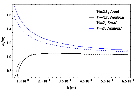
Figure 4 Validation for local⁷⁰ and non-local (present) theory in S-S boundary conditions And also, for the C-C boundary condition:

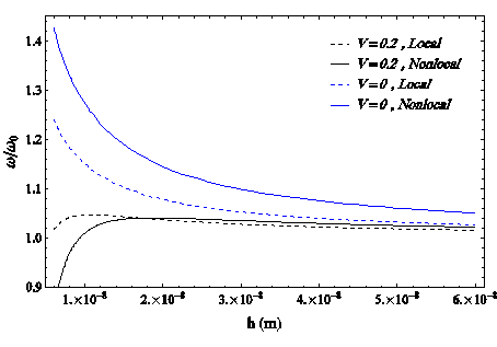
Figure 5 Validation for local⁷⁰ and non-local (present) theory in C-C boundary conditions
Furthermore, for the other forms of the surface effects:
Form 1:${\sigma }_x^0\ne 0,c_{11}^s\ne 0,e_{31}^s\ne 0$
Form 2:${\sigma }_x^0=0,c_{11}^s=0,e_{31}^s=0$
Form 3:${\sigma }_x^0\ne 0,c_{11}^s=0,e_{31}^s=0$
Form 4:${\sigma }_x^0=0,c_{11}^s\ne 0,e_{31}^s=0$

Figure 6 Validation for various forms of surface effects in S-S boundary conditions

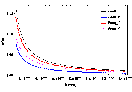
Figure 7 Validation for various forms of surface effects in C-C boundary conditions.

1. The effect of non-local parameter and electric-magnetic fields

In the below curves, the changes of dimensionless frequency of the free oscillations at the first mode with two different boundary conditions in terms of the applied voltage and different values of dimensionless non-local parameter, with input parameters ${\sigma }_x^0=1,H_x=0,C_0=0,K_1=10$ , are shown.

Figure 8 The dimensionless frequency change curve of the free oscillations of the first mode of the system in terms of the applied voltage for different values of the dimensionless non-local parameter of the nanotube, in SS boundary conditions.

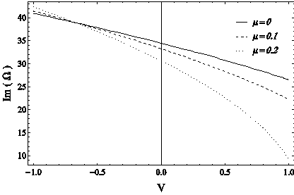
Figure 9 The dimensionless frequency change curve of the free oscillations of the first mode of the system in terms of the applied voltage for different values of the dimensionless non-local parameter of the nanotube, in CC boundary conditions.

In the below curves, the frequency changes of dimensionless free oscillations at the first mode of free vibration of the linear system for two different boundary conditions according to the magnitude of the applied magnetic field in different values of dimensionless non-local parameter, with input parameters ${\sigma }_x^0=1,V=0.5,C_0=0,K_1=10$ , are shown.

Figure 10 The dimensionless frequency change curve of the free oscillations of the first mode of the system in terms of the magnitude of the magnetic field for different values of the dimensionless non-local parameter of the nanotube, in SS boundary conditions.

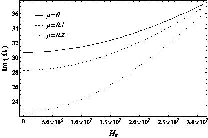
Figure 11 The dimensionless frequency change curve of the free oscillations of the first mode of the system in terms of the magnitude of the magnetic field for different values of the dimensionless non-local parameter of the nanotube, in CC boundary conditions.

2. Effect of hardness-linear damping parameters of viscoelastic foundation

In the below curves, the frequency changes of the dimensionless free oscillations at the first mode of the free vibration of the linear system for two different boundary conditions according to the magnitude of the linear stiffness of the foundation in different forms considering surface effects, with input parameters ${\sigma }_x^0=1,H_x=1\times {10}^7,\mu =0.1,C_0=0,V=1$ , are shown.

Figure 12 The dimensionless frequency change curve of free oscillations of the first mode of the system in terms of dimensionless linear stiffness of the substrate for different forms considering surface effects, in SS boundary conditions.

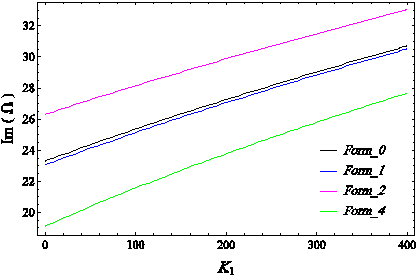
Figure 13 The dimensionless frequency change curve of free oscillations of the first mode of the system in terms of dimensionless linear stiffness of the substrate for different forms considering surface effects, in SS boundary conditions.

In the below curves, the frequency changes of the dimensionless free oscillations at the first mode of the free vibration of the linear system for two different boundary conditions according to the linear damping coefficient of the foundation in different forms considering surface effects, with input parameters ${\sigma }_x^0=1,H_x=1\times {10}^7,\mu =0.1,K_1=100,V=0.5$ , are shown.

Figure 14 The dimensionless frequency change curve of real and imaginary parts of the special values of the first mode of the system in terms of dimensionless linear damping of the substrate for different forms considering surface effects, in SS boundary conditions.

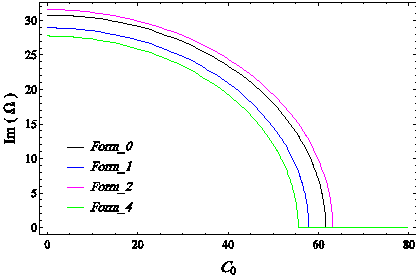
Figure 15 The dimensionless frequency change curve of real and imaginary parts of the special values of the first mode of the system in terms of dimensionless linear damping of the substrate for different forms considering surface effects, in CC boundary conditions.

In the below curves, the results of the nonlinear vibration for the non-damped system are presented.

For $H_x=0,\mu =0.1,K_3=100,V=0.5$ :

Figure 16 Graph of Nonlinear Frequency to Linear Frequency Ratio of the Immortal System Base Mode for Different Values of the foundation Linear Hardness Parameter, Left: SS boundary condition, right: CC boundary condition.

For $H_x=0,\mu =0.1,K_1=100,K_3=100$ :

Figure 17 Graph of Nonlinear to Linear Frequency Ratio Changes of the Immortal System Base Mode for Different Values of Applied Voltage, Left: SS Boundary Conditions, Right: CC Boundary Conditions.

For $\mu =0.1,K_1=100,K_3=100,V=0.5$ :

Figure 18 Graph of Nonlinear Frequency to Linear Frequency Ratio of the Immortal System Base Mode for Different Values of Applied Magnetic Field, Left: SS Boundary Conditions, Right: CC Boundary Conditions.

For ${\text{H}}_{\text{x}}=1\times {10}^7,{\text{K}}_1=100,{\text{K}}_3=100,\text{V}=0.5$  

Figure 19 Graph of changes in the ratio of nonlinear to linear frequency ratio of the base mode of the immortal system for different values of the non-local parameter of the nanotube, left: SS boundary condition, right: CC boundary condition.

In the following two diagrams for zero voltage and negative voltage, nonlinear to linear frequency ratio diagrams are drawn for SS boundary conditions:

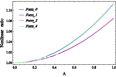
Figure 20 Graph of Nonlinear Frequency to Linear Frequency Ratio of Immortal System Base Mode for Different Forms Considering Surface Effects without Voltage Applied to SS Boundary Conditions.

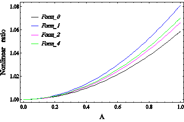
Figure 21 Graph of changes in the ratio of nonlinear to linear frequency ratio of the base mode of the immortal system for different forms Considering surface effects with applied voltage V = -0.5, for SS boundary conditions.

For $\text{V}=0,{\text{H}}_{\text{x}}=0,{\text{K}}_1=0,{\text{K}}_3=50,{\text{C}}_0=0.15,{\text{C}}_2=0,\overline{{\text{x}}_0}=0.5$ :

Figure 22 Amplitude-frequency vibration curves for different values of μ (μ = 0 simple line, μ = 0.2 bold fold line); Figure above: SS boundary conditions, bottom figure: CC boundary conditions.

For $\text{V}=0,{\text{H}}_{\text{x}}=0,{\text{K}}_1=0,{\text{K}}_3=50,{\text{C}}_0=0.15,\text{μ}=0.1,\overline{{\text{x}}_0}=0.5$ :

$V=0, H_x=0, K_1=0,K_3=50, C_0=0.15, \mu =0.1, {\overline{x}}_0=0.5:$

Figure 23 Amplitude-frequency vibration curves for different values of C_2, (C_2 = 1 simple line, C_2 = 3 bold fold lines), Figure above: SS boundary conditions, bottom figure: CC boundary conditions.

For $\text{V}=0,{\text{H}}_{\text{x}}=0,{\text{K}}_1=0,{\text{K}}_3=50,{\text{C}}_2=1,\text{μ}=0.1,\overline{{\text{x}}_0}=0.5$ :  

$V=0, H_x=0, K_1=0,K_3=50, C_2=1, \mu =0.1, {\overline{x}}_0=0.5:$

Figure 24 Amplitude-frequency vibration curves for different values of C_0, (C_0 = 0.1 simple line, C_0 = 0.3 bold fold line), high: SS boundary conditions, low: CC boundary conditions.

For ${\text{H}}_{\text{x}}=0,{\text{K}}_1=100,{\text{K}}_3=50,{\text{C}}_0=0.1,{\text{C}}_2\text{=1,} \text{μ}=0.1,\overline{{\text{x}}_0}=0.5$ :

$H_x=0, K_1=100,K_3=50, C_0=0.1, C_2=1, \mu =0.1, {\overline{x}}_0=0.5:$

Figure 25 Amplitude-frequency vibration curves for different values of V, (V = -0.5 purple line, V = 0 blue fold line, V = 0.5 bold black), high: SS boundary conditions, low: CC boundary conditions.

According to the presented diagrams, the presence of a non-local parameter has increased the curvature deviation to the right and the stiffening effect. In other words, the non-local parameter is a factor to increase the nonlinear effect of the system. On the other hand, the presence of this factor reduces the maximum range of fluctuations.

By comparing the graphs related to two different boundary conditions, the following results are inferred:

1. At the C-C boundary conditions, the diagram is collected and the amount of deviation to the right is reduced. For example, the deviation parameters for the maximum dynamic response for the S-S and C-C boundary condition are 0.065 and 0.0045, respectively. In addition, the dynamic response decreases with less degrees of freedom in boundary conditions. For example, in these diagrams, the maximum dynamic range for S-S and C-C are 0.79 and 0.26, respectively. Also, the damping of the system has a greater effect in the boundary conditions of C-C and has significantly reduced the sharpness of the diagram. Therefore, for the C-C boundary conditions, the effect of substrate damping in reducing the dynamic response at excitation frequencies close to the resonant state of the system was greater.
2. The higher the foundation attenuation, the lower the amplitude of the amplitude-frequency curve, and consequently the lower the maximum dynamic response. Of course, it should be noted that the amplitude-excitation frequency curve for a system with C-C boundary conditions is more sensitive to the damping changes of the foundation than the amplitude-frequency curve of the system excitation of the S-S boundary conditions.
3. As the nonlinear hardness coefficient of the substrate increases, the amplitude-frequency curve deviates to the right, but the maximum dynamic response amplitude remains constant. By looking more closely at the two diagrams, it could be found that the effect of this parameter on deviating of the diagram is greater for S-S boundary conditions due to more flexibility, so the dynamic response in the CC boundary condition is less sensitive to the increasing nonlinear foundation stiffness parameter.
4. According to the obtained results, increasing the linear stiffness of the substrate has led to a decrease in the dynamic response as well as the peak deviation of the curve. Increasing the linear stiffness of the system reduces the nonlinear effects of the system. In addition, in the C-C boundary conditions, where the overall stiffness of the system is higher, this factor is less effective.
5. The presence of a magnetic factor, in addition to reducing the amplitude of the dynamic response, has led to a decrease in the amplitude of the peak and also a reduction in its curvature to the right. However, these effects have attracted more attention for S-S boundary conditions, which have a more flexible system than for C-C boundary conditions.
6. According to the curves, it is quite clear that by changing the applied voltage from zero to a positive value, the response amplitude has increased sharply and the deviation to the right has increased as well. However, by changing the voltage from zero to a negative value, both the dynamic response amplitude and the peak deviation of the graph are reduced as well as nonlinear effects of the system. It is also important to note that under the same conditions these changes for C-C boundary conditions are much less than for S-S boundary conditions and in general it could be said that the sensitivity of the dynamic response curve of the system with C-C boundary condition to most investigated changes in the system input parameters such as foundation stiffness, voltage, and magnetic factor, non-local factor and surface effects are less than the sensitivity of the system with SS boundary conditions.
7. It could be seen that by considering the parameter of residual surface stresses for the system, the response amplitude, and the amount of curvature deviation to the right are reduced.
8. It is predictable that as the load affect position moves away from the center of the wire toward the supports, the amplitude of the dynamic response decreases significantly, and this relative reduction is greater for the C-C boundary condition than for the S-S boundary condition. It is also important to note that the location of the load has no effect on the rate of deviation of the curve peak and the degree of nonlinearity of the dynamic response of the system.
9. Given that the voltage applied to the system is positive for the last two numerical diagrams. It is expected that the graph with the highest deviation and the lowest peak amplitude is related to Form 4 and the graph with the lowest deviation and the lowest peak amplitude is also related to Form 2. In addition, in this case, by comparing the two curves of Form 1 and the main form, it can be concluded that by considering the surface parameters (Form 1), the maximum peak amplitude and the deviation of the graph have increased.

None.

None.

The authors declare that they have no competing interests.

1. Maziar J, Zare A. Free vibration analysis of functionally graded carbon nanotubes with variable thickness by differential quadrature method. Physica E: Low-Dimen Sys Nanostruc. 2011;43(9):1602–1604. ‏
2. Manbachi A, Cobbold RSC. Development and application of piezoelectric materials for ultrasound generation and detection. Ultrasound. 2011;19(4):187–196. ‏
3. Zhi Y, Jiang L. Surface effects on the electromechanical coupling and bending behaviours of piezoelectric nanowires. J Phys D Appl Phys. 2011;44(7):075404. ‏
4. Zhi Y, Jiang L. Surface effects on the electroelastic responses of a thin piezoelectric plate with nanoscale thickness. J Phys D Appl Phys. 2021;45(25):255401. ‏
5. Zhengrong Z, Jiang L. Size effects on electromechanical coupling fields of a bending piezoelectric nanoplate due to surface effects and flexoelectricity. J Appl Phys. 2014;116(13):134308. ‏
6. Issa B, Obaidat IM, Albiss BA, et al. Magnetic nanoparticles: surface effects and properties related to biomedicine applications. Int J Mol Sci. 2013;14(11):21266–21305. ‏
7. Assadi A. Size dependent forced vibration of nanoplates with consideration of surface effects. Appl Math Model. 2013;37(5):3575–3588. ‏
8. Wu JX, Li XF, Tang AE, et al. Free and forced transverse vibration of nanowires with surface effects. J Vibrat Control. 2017;23(13):2064–2077. ‏
9. Malikan M, Nguyen VB, Tornabene F. Damped forced vibration analysis of single-walled carbon nanotubes resting on viscoelastic foundation in thermal environment using nonlocal strain gradient theory. Eng Sci Tech Int J. 2018;21(4):778–786.
10. Zarezadeh E, Hosseini V, Hadi A. Torsional vibration of functionally graded nano-rod under magnetic field supported by a generalized torsional foundation based on nonlocal elasticity theory. Mech Based Design Struct Mach. 2020;48(4):480–495.
11. Zhen YX, Wen SL, Tang Y. Free vibration analysis of viscoelastic nanotubes under longitudinal magnetic field based on nonlocal strain gradient Timoshenko beam model. Physica E: Low-Dimen Sys Nanostruc. 2019;105:116–124.
12. Lee H, Chang WJ. Vibration analysis of a viscous-fluid-conveying single-walled carbon nanotube embedded in an elastic medium. Physica E: Low-Dimen Sys Nanostruc. 2009;41(4):529–532.
13. Kiani K. Vibration analysis of elastically restrained double-walled carbon nanotubes on elastic foundation subject to axial load using nonlocal shear deformable beam theories. Int J Mech Sci. 2013;68:16–34.
14. Aydogdu M. Axial vibration analysis of nanorods (carbon nanotubes) embedded in an elastic medium using nonlocal elasticity. Mech Res Commun. 2012;43:34–40.
15. Wang BL, Wang KF. Vibration analysis of embedded nanotubes using nonlocal continuum theory. Compos B Eng. 2013;47:96–101.
16. Ke LL, Xiang,Y, Yang J, et al. Nonlinear free vibration of embedded double-walled carbon nanotubes based on nonlocal Timoshenko beam theory. Comput Mater Sci. 2009;47(2):409–417.
17. Fang B, Zhen YX, Zhang CP, et al. Nonlinear vibration analysis of double-walled carbon nanotubes based on nonlocal elasticity theory. Appl Math Model. 2013;37(3):1096–1107.
18. Simsek M. Nonlocal effects in the forced vibration of an elastically connected double-carbon nanotube system under a moving nanoparticle. Comput Mater Sci. 2011;50(7):2112–2123.
19. Ansari R, Ramezannezhad H. Nonlocal Timoshenko beam model for the large-amplitude vibrations of embedded multiwalled carbon nanotubes including thermal effects. Physica E: Low-Dimen Sys Nanostruc. 2011;43(6):1171–1178.
20. Ansari R, Ramezannezhad H, Gholami R. Nonlocal beam theory for nonlinear vibrations of embedded multiwalled carbon nanotubes in thermal environment. Nonlinear Dyn. 2012;67:2241–2254.
21. Kiani K. A meshless approach for free transverse vibration of embedded single walled nanotubes with arbitrary boundary conditions accounting for nonlocal effect. Int J Mech Sci. 2010;52(10):1343–1356.
22. Murmu T, Pradhan SC. Thermo-mechanical vibration of a single-walled carbon nanotube embedded in an elastic medium based on nonlocal elasticity theory. Comput Mater Sci. 2009;46(4):854–859.
23. Chang TP. Thermal–mechanical vibration and instability of a fluid-conveying single-walled carbon nanotube embedded in an elastic medium based on nonlocal elasticity theory. Appl Math Model. 2012;36(5):1964–1973.
24. Rahmati AH, Mohammadimehr M. Vibration analysis of non-uniform and non-homogeneous boron nitride nanorods embedded in elastic medium under combined loadings using DQM. Physica B Condensed Matter. 2014;440:88–98.
25. Pradhan SC, Reddy GK. Buckling analysis of single walled carbon nanotube on Winkler foundation using on nonlocal elasticity theory and DTM. Comput Mater Sci. 2011;50(3):1052–1056.
26. Narender S, Gopalakrishnan S. Critical buckling temperature of single walled carbon nanotubes embedded in a one-parameter elastic medium based on nonlocal continuum mechanics. Physica E: Low-Dimen Sys Nanostruc. 2011;43(6):1185–1191.
27. Murmu T, Pradhan SC. Thermal effects on the stability of embedded carbon nanotubes. Comput Mater Sci. 2010;47(3):721–726.
28. Arani AG, Amir S, Shajari AR, et al. Electro-thermal nonlocal vibration analysis of embedded DWBNNTs. Proc Inst Mech Eng C J Mech Eng Sci. 2011;224(5):745–756.
29. Mikhasev G. On localized modes of free vibrations of single walled carbon nanotubes embedded in nonhomogeneous elastic medium. ZAMM J Appl Math Mech. 2014;94(1–2):130–141.
30. Fu YM, Hong JW, Wang XQ. Analysis of nonlinear vibration for embedded carbon nanotubes. J Sound Vib. 2006;296:746–756.
31. Komijani M, Esfahani SE, Reddy JN, et al. Nonlinear thermal stability and vibration of pre/post-buckled temperature and microstructure dependent functionally graded beams resting on elastic foundation. Compos Struct. 2014;112:292–307.
32. Ozturk B, Coskun SB, Koc MZ, et al. Homotopy perturbation method for free vibration analysis of beams on elastic foundation. IOP Conf Ser Mater Sci Eng. 2010;10(1):012158.
33. Öz HR, Pakdemirli M, Özkaya E, et al. Nonlinear vibrations of a slightly curved beam resting on a nonlinear elastic foundation. J Sound Vib. 1998;212:295–309.
34. Yan Y, Wang,W, Zhang L. Applied multiscale method to analysis of nonlinear vibration for double walled carbon nanotubes. Appl Math Model. 2011;35(5):2279–2289.
35. Bagdatlı SM. Non-linear vibration of nanobeams with various boundary condition based on nonlocal elasticity theory. Compos B Eng. 2015;80:43–52.
36. Bagdatlı SM. Non-linear transverse vibrations of tensioned nanobeams using nonlocal beam theory. Struct Eng Mech. 2015;55(2):281–298.
37. Eringen AC, Wegner JI. Nonlocal continuum field theories. Appl Mec Rev. 2003;56(2):B20–B22.
38. Zhang Y, Liu GR, Xie XY. Free transverse vibrations of double-walled carbon nanotubes using a theory of nonlocal elasticity. Phys Rev B. 2005;71(19):195404.
39. Sudak L. Column buckling of multiwalled carbon nanotubes using nonlocal continuum mechanics. J Appl Phys. 2003;94(11):7281–7287.
40. Azarboni HR. Magneto-thermal primary frequency response analysis of carbon nanotube considering surface effect under different boundary conditions. Composite Part B: Eng. 2019;165:435–441.
41. Ghayesh Mergen H. Nonlinear size-dependent behaviour of single-walled carbon nanotubes. Applied Physics A. 2014;117(3):1393–1399. ‏
42. Zhen Ya-Xin, Fang Bo. Nonlinear vibration of fluid-conveying single-walled carbon nanotubes under harmonic excitation. International Journal of Non-Linear Mechanics. 2015;76:48–55. ‏
43. Mahdavi M H, Jiang L Y, Sun X. Nonlinear vibration of a single-walled carbon nanotube embedded in a polymer matrix aroused by interfacial van der Waals forces. Journal of Applied Physics. 2009;106(11):114309. ‏
44. Huang Kun, Zhang S, Li J, et al. Nonlocal nonlinear model of Bernoulli–Euler nanobeam with small initial curvature and its application to single-walled carbon nanotubes. Microsystem Technologies. 2019;25(11):4303–4310. ‏
45. Huang Kun, Qu B, Xu W, et al. Nonlocal Euler–Bernoulli beam theories with material nonlinearity and their application to single-walled carbon nanotubes. Nonlinear Dynamics. 2022;109(3):1423–1439. ‏
46. Setoodeh AR, Khosrownejad M, Malekzadeh P. Exact nonlocal solution for postbuckling of single-walled carbon nanotubes. Physica E: Low-dimensional Systems and Nanostructures. 2011;43(9):1730–1737. ‏
47. Wang Bo, Deng Z, Zhou J, et al. Wave propagation analysis in nonlinear curved single-walled carbon nanotubes based on nonlocal elasticity theory. Physica E: Low-dimensional Systems and Nanostructures. 2015;66:283–292. ‏
48. Narendar S, Gupta S S, Gopalakrishnan S. Wave propagation in single-walled carbon nanotube under longitudinal magnetic field using nonlocal Euler–Bernoulli beam theory. Applied Mathematical Modelling. 2012;36(9):4529–4538. ‏
49. Hosseini M, Bahaadini R, Jamali B. Nonlocal instability of cantilever piezoelectric carbon nanotubes by considering surface effects subjected to axial flow. Journal of Vibration and Control. 2018;24(9):1809–1825. ‏
50. Shahsavari S, Allafchian A, Torkaman P, et al. Vibration Analysis of Piezoelectric Carbon Nanotube Considering Surface Effects, Located in the Magnetic Field and Resting on Nonlinear Viscoelastic Foundation. Nanobiotechnology Reports. 2022;17:64–73.
51. Gheshlaghi B, Hasheminejad Seyyed M. Vibration analysis of piezoelectric nanowires with surface and small scale effects. Current applied physics. 2012;12(4):1096–1099. ‏
52. Amiri Ahad, Vesal Rahim, Talebitooti Roohollah. Flexoelectric and surface effects on size-dependent flow-induced vibration and instability analysis of fluid-conveying nanotubes based on flexoelectricity beam model. International Journal of Mechanical Sciences. 2019;156:474–485. ‏
53. Gia Phi B, Van Hieu D, Sedighi H M, et al. Size-dependent nonlinear vibration of functionally graded composite micro-beams reinforced by carbon nanotubes with piezoelectric layers in thermal environments. Acta Mechanica. 2022;233:2249–2270.
54. Zheng Ting X, Ming Li C. Single cell analysis at the nanoscale. Chemical society reviews. 2012;41(6):2061–2071. ‏
55. Kalweit M. Molecular modelling of meso-and nanoscale dynamics. 2008. ‏
56. Zhang Luzheng, Jiang Shaoyi. Molecular simulation study of nanoscale friction for alkyl monolayers on Si (111). The Journal of Chemical Physics. 2002;117(4):1804–1811. ‏
57. Kosloff Ronnie. Time-dependent quantum-mechanical methods for molecular dynamics. J Phys Chem. 1988;92(8):2087–2100. ‏
58. Sullivan Dennis M, Citrin D S. Determining quantum eigenfunctions in three-dimensional nanoscale structures. Journal of Applied Physics. 2005;97(10):104305. ‏
59. McCarthy Robert. System, Method, and Product for Nanoscale Modeling, Analysis, Simulation, and Synthesis (NMASS). U.S. Patent Application No. 10/248,092. ‏ 2003.
60. Anantram M P, Lundstrom M S, Nikonov D E. Modeling of nanoscale devices. Proceedings of the IEEE 96.9. 2008:1511–1550. ‏
61. Eringen AC. On differential-equations of nonlocal elasticity and solutions of screw dislocation and surface-waves. J Appl Phys. 1983;54(9):4703–4710.
62. Eringen AC. Nonlocal Continuum Field Theories; Springer-Verlag: New York, NY, USA, 2002.
63. Karaoglu P, Aydogdu M. On the forced vibration of carbon nanotubes via a non-local Euler—Bernoulli beam model. Proceedings of the Institution of Mechanical Engineers, Part C: Journal of Mechanical Engineering Science. 2010;224(2):497–503. ‏
64. Kemp B A, Grzegorczyk T M, Kong J A. Lorentz force on dielectric and magnetic particles. Journal of electromagnetic waves and applications. 2006;20(6):827–839. ‏
65. Dingreville Rémi, Qu Jianmin, Cherkaoui Mohammed. Surface free energy and its effect on the elastic behavior of nano-sized particles, wires and films. Journal of the Mechanics and Physics of Solids. 2005;53(8):1827–1854. ‏
66. Diao Jiankuai, Gall Ken, Dunn Martin L. Surface-stress-induced phase transformation in metal nanowires. Nature materials. 2003;2(10):656–660. ‏
67. Rehm Warren S. The effect of electric current on gastric secretion and potential. American Journal of Physiology-Legacy Content. 1945;144(1):115–125. ‏
68. Il’ina Marina V, Il’ina O I, Blinov Y F, et al. Piezoelectric response of multi-walled carbon nanotubes. Materials. 2018;11(4):638. ‏
69. Yan Z, Jiang L Y. The vibrational and buckling behaviors of piezoelectric nanobeams with surface effects. Nanotechnology. 2011;22(24):245703. ‏
70. McCarthy Robert. System, Method, and Product for Nanoscale Modeling, Analysis, Simulation, and Synthesis (NMASS). U.S. Patent Application No. 10/248,092. ‏ 2003.