Presentation of jute fibre length via graphics and computer simulation with gamma distribution function

doi:10.15406/jteft.2017.02.00058

Journal of

eISSN: 2574-8114

Textile Engineering & Fashion Technology

Review Article Volume 2 Issue 3

Presentation of jute fibre length via graphics and computer simulation with gamma distribution function

SK Biswas

Verify Captcha

Regret for the inconvenience: we are taking measures to prevent fraudulent form submissions by extractors and page crawlers. Please type the correct Captcha word to see email ID.

Department of Jute and Fibre Technology, University of Calcutta, India

Correspondence: SK Biswas, Textile Physics Section, Department of Jute and Fibre Technology, Institute of Jute Technology, University of Calcutta 35, Ballygunge Circular Road, Calcutta-700019, India, Tel 943228483

Received: January 25, 2017 | Published: July 18, 2017

Citation: Biswas SK. Presentation of jute fibre length via graphics and computer simulation with gamma distribution function. J Textile Eng Fashion Technol. 2017;2(3):370-374. DOI: 10.15406/jteft.2017.02.00058

Download PDF

Abstract

Notwithstanding the complexity of production of jute fibre filaments a simple graphical presentation of jute fibre length distribution is made. The computer simulation of four types of frequency distribution of jute fibre length depending on method of sampling and testing is presented. These four distribution curves give six points of intersections which merit technological significance. A study of fibre length-frequency distribution depending on methods of sampling and testing may lead to a general form of Gamma distribution function. The parameters in the mathematical formulae may serve as characteristics of condition giving the benchmark for valid experiment. This type of work involving exponential distribution was not done previously and provides a deeper insight into the characterisation of its comparative features with respect to normal distribution of fibre length.

Keywords: gamma distribution, jute fibre, fibre length, length distribution

Introduction

In jute, the raw fibre as it comes from the plant consists of many single filaments bonded together by adhesion and branching to form a three-dimensional meshy structure. On carding, this meshy structure is broken into individual fibrous elements of different lengths , the longer elements being more complex, since these consists of several single filament still joined together in some way. This complexity will cause the linear density of the longer elements to be greater than that of the single filaments. In addition, the single filaments in the longer elements may be thicker and stronger than those in the shorter ones. On both these counts, the linear density of the longer elements will be greater than that of the shorter ones Banerjee.¹ When the meshy structure of raw jute reeds is broken down randomly into fibrous elements in a carding machine, the frequency of such elements by number can be expected to decrease exponentially with increase in their length Banerjee.² In this paper a graphical presentation of jute fibre length distribution is made.

A study of fibre length-frequency distribution depending on methods of sampling and testing may lead to a general form of Gamma distribution function. It may be mentioned that for Gamma distribution Trivedi³ the density function of the random variable x is given by

$f_{x} (x) = (1 / (Γ α)) (λ^{α} x^{α - 1} e^{- λ x}), α \geq 0$ (1)

Whose mean=α/λ, variance = α/λ₂, standard deviation = $\sqrt{α} / λ$ and coefficient of variation = $100 / \sqrt{α}$ . This distribution has two parameters. The parameter α is called a shape parameter since, as α increases, the density becomes more peaked. The parameter λ is a scale parameter; that is, the distribution depends on λ only. Variation for the values of α which May serves as behavior characteristic of condition that appears as parameters in the mathematical formulae giving the benchmark for valid experiment.

Presentation of fibre length via graphics

Figure 1 is the graphical representation of data collected by measuring length of single fibres. The vertical axis is number (quantity) of fibre, the horizontal axis fibre length increments, and each circle o, represents a single fibre. One could imagine that the o‘s are end views fibres stacked vertically with each stack consisting only of fibres of same length. To the left hand side are the short fibres, the right hand side the long fibres. Statisticians call Figure 1 a histogram or length frequency distribution diagram. Figure 1 gives all of the information we need to know about fibre length and fibre length distribution. Since it is easier to determine the weight of fibre than to count the number of fibre, histograms and staple diagrams (arrays) are usually constructed on fibre weight basis. For clarity and ease of explanation, fibre number basis is used in this discussion. Detailed discussion about number and weight basis of testing is made in later section of this paper. Another method of representing data collected by measuring length of fibres is in Figure 2a. The vertical axis is number (quantity) of fibre, the horizontal axis is the fibre length and each cylinder represents a fibre. Figure 2a is a picture of fibres arranged in order of length with left hand ends aligned at the vertical axis. Figure 2a is simply a rearrangement of Figure 1 & 2a is the staple diagram and, as in Figure 1, contains all of the information we need to know about end to end lengths.

Figure 1 Histogram.

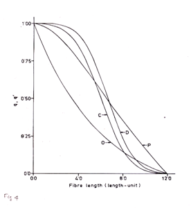
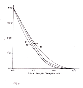
Millions of millions of fibres are involved in fibre and yarn production. (Figures 1)(Figures 2a) do not contain all the fibres, they contain only a representative number of fibres. More realistic is Figure 2b which is three dimensional having a z-axis. Layer after layer of staple diagrams on to infinity. A bale of fibres could be represented as in Figures 2b. As fibres were rearranged going from Figures 1 to Figures 2a so can the fibres be rearranged as illustrated in Figures 3. To make this rearrangement, fibres of Figures 2b are selected at random along their lengths, the catch points placed on the vertical axis, and fibres thus selected arranged in descending order of the extension distance to the right hand side of the catch point. For illustration, fibre segments marked 1, 2, & 3 in Figures 2b are shown in their appropriate location in Figures 3, accordingly enough fibres are selected to make the Figures 3 becomes representative. Figures 3 is a Fibrogram and contains all of the information we need to know about fibre length and fibre length distribution Of the three methods of representative of fibre length, the staple diagram of Figures 2a is easily accepted by our mental processes, the mental picture requires no strain on the imagination and we have a comfortable feeling; thus the staple diagram has been established as the standard of comparison and the bench mark from which other fibre length test methods are compared.⁴ However, in yarn spinning and non-woven fabric production, ends of fibres must never be aligned. The Fibrogram which is an arrangement of fibre as they are, or as they will be in future processes, becomes the bench mark of comparison concerning fibre performance in yarn spinning and non-woven fabric manufacture⁴ This type of work involving exponential distribution was not done previously and provides a deeper insight into the characterisation of its comparative features with respect to normal distribution of fibre length. The survivor diagrams (curves O and P) and fibrograms (curves Q and R) are also computed and presented in Figure 4 for end-biased and length-biased samples respectively. It can be observed from Figure 5 that fibrograms for exponential and normal distributions have close similarity if their mean values are same. This is corroborated with the values of the corresponding fibrogram parameters. However the survivor or array diagram which is also still popular in industrial practice distinguishes the basic distributions as evident in Figure 4, better than the fibrogram. This would be useful in the context that the basic frequency distributions of fibre lengths are somewhat difficult to obtain from direct experiments.

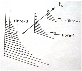
Figure 2 a: Total population, b: Stable diagram.

Effect of sampling and testing method

In fibre length measurements two kinds of sample are experimentally obtainable through two kinds of sampling methods-end-biased and length biased. An end-biased sample is defined as one in which each fibre of population has equal probability of being included since each fibre has two ends independent of its length or any other characteristics. The end-biased sample is a random sample. A length-biased sample is one in which the probability of a fibre being included is directly proportional to its length. In fibre testing, a random selection is restricted due to the essential nature of the fibre that it is much longer than it is thick. Because of this, it is only too easy to take a sample in such a way that it contains far more long fibres than it should. The knowledge of the nature of bias in favour of the longer fibre would help to avoid the same. In some contexts in which length biased sampling is used it is reasonable to regard the length biased distribution as the object of study Cox.⁵ The frequency distributions of fibre length in jute slivers and yarns have been deduced analytically by Banerjee² for different methods of sample preparation. The expected average length of fibres obtained on the basis of number and weight of fibres has been estimated for each of such distribution. The present author Biswas^6-8 has shown that the Gamma function provides mathematical short-cut for the analysis of fibre length distribution and average length of jute fibres depending on sampling and testing method to arrive at the results as obtained by Banerjee. The two sampling method i.e., (i) end-biased and (ii) length biased sampling method have been considered. For each of such sampling the expected distribution of fibre length obtained on the basis of (i) number and (ii) weight of fibres has also been estimated. Thus four types of length distributions are obtained such as the frequency of length l tested on the basis of number from end-biased sample (f_EN (l)), the frequency of fibre of length l tested on the basis of number from a length-biased sample (f_LN (l)), the frequency of fibre of length l tested on the basis of weight from an end-biased sample (f_EW (l)) and the frequency of fibre of length l tested on the basis of weight from a length biased sample (f_LW (l)).

Figure 3 Fibrogram.

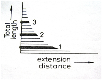
Figure 4 Theoretical Survivor diagrams of cotton fibre of 6 length-unit mean fibre length and12 length-unit maximum fibre length on the basis of number from an end- biased sample (curve-C) and length-biased sample (curve-D); and jute fibre in sliver and yarns of 6 length-unit mean fibre length and 12 length-unit maximum fibre length on the basis of number from an end-biased sample (curve-O) and length-biased sample (curve-P).

Figure 5 Theoretical Fibrograms of cotton fibre of 6 length-unit mean fibre length and12 length-unit maximum fibre length on the basis of number from an end- biased sample(curve- E) and length-biased sample (curve-F); and jute fibre in sliver and yarns of 6 length-unit mean fibre length and 12 length-unit maximum fibre length on the basis of number from an end-biased sample(curve- Q) and length-biased sample (curve- R).

Figure 6 Theoretical length distribution of jute fibres in yarns and slivers. (A-end-biased number based method; B-length biased number based method; C-end-biased weight based method; and D-length-biased weight based method).

The end-biased and number based length distribution of fibre f_EN (l), which is expected to be similar to the basic type has been used by Banerjee² to obtain f_LN (l) and f_EW (l), and in turn f_LN (l) has been used to obtain f_LW (l). The present author uses the Gamma function to obtain the same result very quickly Biswas^6-8 and f_EW (l) has been considered Biswas¹ to obtain f_LW (l). He has also considered all the other possible routes of transformations of one type of length distribution to the other types of length distribution and presented their rederivation through Gamma function to achieve a considerable simplification Biswas.⁹ The summary of the results of the distribution is given in Table 1. Cox⁵ describes relations between mean (µ) of the end-biased distribution f(x) and an expectation (mean or average) Eg(x) with respect to length-biased distribution g(x) as $E g (X) = μ [1 + \frac{σ 2}{μ 2}]$ Where µ, α are the mean and standard deviation of the end-biased distribution f(x). For Gamma distribution the above relation becomes $E g (X) = \frac{1}{λ} (1 + α)$ Where α is called a shape parameter of the end-biased distribution f(x).

Method Followed	Relationship for Frequency Distribution	Average Length
Basic population number-based	$f (l) = \frac{1}{l^{-}} \exp (- l / l^{-})$	$^{-} l$
End-biased sampling number-based	$f_{E N} (l) = \frac{1}{l^{-}} \exp (- l / l^{-})$	$^{-} l$
Length-biased sampling number-based	$f_{L N} (l) = \frac{1}{l^{-}^{2}} \exp (- l / l^{-})$	$2 {}^{-}l$
End-biased sampling weight-based	$f_{E N} (l) = \frac{l^{2}}{l^{-}^{3}} \exp (- l / l^{-})$	$3 {}^{-}l$
Length-biased sampling weight-based	$f_{L W} (l) = \frac{l^{3}}{l^{-}^{4}} \exp (- l / l^{-})$	$4 {}^{-}l$

Table 1 Summary of results of derivation

Computer simulation & modal length

The computer simulations of four frequency distribution function f_EN(l), f_LN(l), f_EW(l) and f_LW(l) as given in Table 1 were carried for l=5 cm. The computer programme in F77 is given in Appendix-1. The resulting curves obtained with the help of a Graphic Software are presented in Figure 6. However the proliferation of so many distribution curves depending on the method of sampling and testing may give several points of intersection when these are superimposed. In fact reports of experimental observation of intersection were available in some cases and attempt had been made to attribute suitable technological significance to it Sinha,^10,11 Biswas & Chanda.⁴ The present author Biswas¹² has found out analytically all the intersections and showed that intersections depend on the average length of fibre population. Computer simulations are also presented and reported here. He has also found out analytically the modal length of fibre length-frequency distribution depending on methods of sampling and testing Biswas.^13,14 The best measure of staple length for general application is given by modal or most frequent length of fibre length- frequency distribution Morton & Hearle.¹⁵ The modal length $l^{m}$ can be determined from the condition Goon et al.¹⁶ at x = $l^{m}$ (2)

Using Equation (1), Equation (2) can be written as

$((α - 1) x^{α - 2} e^{- λ x} - λ x^{α - 1} e^{- λ x}) = 0$

$l^{m} = \frac{(α - 1)}{λ}$ (3)

Motivation and conclusion

It may be mentioned that for Gamma distribution the density function of the random variable x is given

by $f_{x} (x) = (1 / (Γ α)) (λ^{α} x^{α - 1} e^{- λ x}), α \geq 0$

Whose mean = α/λ, variance = α/λ₂, standard deviation $\sqrt{α} / λ$ and coefficient of variation = $100 / \sqrt{α}$ . This distribution has two parameters. The parameter α is called a shape parameter since, as α increases, the density becomes more peaked. The parameter λ is a scale parameter; that is, the distribution depends on λ only. A study of fibre length-frequency distribution depending on methods of sampling and testing in Table 1 may lead to a general form of Gamma distribution function if we use 1/ l =λ. This remains the motivation of this work. Table 2 gives Standard Deviation and Coefficient of Variation for the respective values of α which May serves as behaviour characteristic of condition that appear as parameters in the mathematical formulae giving the benchmark for valid experiment. It may be noted that not only average length of fibre but also standard deviation and coefficient variation depend on methods of sampling and testing. Table 3 gives Summary of Results of average length from Cox’s formula and modal length from equation (3).

Method Followed	Standard Deviation	Coefficient of Variation (%)
Gamma distribution (Shape parameter=α, Scale parameter λ=1/l	$\sqrt{α} / λ$	$100 / \sqrt{α}$
Basic population number-based Where α=1	$^{-} l$	100
End-biased sampling number-based Where α=1	$^{-} l$	100
Length-biased sampling number-based Where α=2	$\sqrt{2} {}^{-}l$	$100 / \sqrt{2} = 71$
End-biased sampling weight-based Where α=3	$\sqrt{3} {}^{-}l$	$100 / \sqrt{3} = 58$
Length-biased sampling weight-based Where α=4	$2 {}^{-}l$	$100 / 2 = 50$

Table 2 Summary of results of standard deviation and coefficient of variation

Method Followed	Average Length from Cox's Formula	Model Length from Equation (3)
Gamma distribution (Shape parameter=α, Scale parameter λ=1/l	$E g (X) = μ [1 + \frac{σ 2}{μ 2}]$	$l m = (α - 1) / λ$
Basic population number-based Where α=1	Not required	0
End-biased sampling number-based Where α=1	Not required	0
Length-biased sampling number-based Where α=2	$2 {}^{-}l$	$^{-} l$
End-biased sampling weight-based Where α=3	$3 {}^{-}l$	$2 {}^{-}l$
Length-biased sampling weight-based Where α=4	$4 {}^{-}l$	$3 {}^{-}l$

Table 3 Summary of results of average length from Cox’s formula and model length form equation (3)

However attempts may be made to attribute suitable technological significance to it (by physically matching fibrograms of various types of fibres considering their distribution parameters of mean, standard deviation, minimum and maximum length). This would be useful guidance concerning fibre performance in yarn processing of blends or mixing of fibres having exponential and normal distributions of their lengths that they should have their mean values being same as well as their respective values of maximum lengths also being same.

References

- Banerjee BL. The relation between the length and linear density of jute and flax fibres obtained after carding and drawing operations. J Textile Inst. 1982;73(4):183‒188.
- Banerjee BL. Effects of sampling and testing methods on the determination of fibre length in jute slivers and yarns. Indian J Fiber & Textile Res. 1980;5(3):98‒102.
- Trivedi KS. Probability & Statistics with Reliability, Queuing, and Computer Science Applications. USA: John Wiley & Sons; 1994.
- Biswas SK, Chanda RS. Mathematical Approach to Generating Fibre Length Distribution via Computer simulation in Jute and allied Fibre: Production, Utilisation and Marketing. In: Palit P, Sinha MK, editors. Indian Fibre Society, Eastern Region, Ghana; 2010. p. 83‒90.
- Cox DR. Some sampling problems in technology. Symposium on the foundation of survey sampling. In: Johnson NL, Smith H, editors. New York: John Wiley; 1969. p. 506.
- Biswas SK. Use of Gamma function in the Calculation of average fibre length. Indian J Fiber & Textile Res. 1989;14(3):145‒146.
- Biswas SK. Some application of Gamma Function in the Calculation of average fibre length Jute Development J. 1990;10:26‒27.
- Biswas SK. Application of Gamma Function in the Determination of fibre length in Jute Slivers and Yarns. Modern Textile Journal. 2010. p. 44‒47.
- Biswas SK. Some studies of jute fibre length distribution with Gamma Function. IAPQR Transations. 1996;21:67‒72.
- Sinha NG. Physical aspect of fine spinning of jute. Indian J Phys. 1975;49:245‒248.
- Sinha NG. Physical conditions for finest and best quality yarns from jute. J Text Assoc. 1975;36:51‒57.
- Biswas SK. Computational and simulation studies of jute fibre length distribution. Indian J Fibre & Text Res. 2000;25(3):221‒224.
- Biswas SK. Computer simulation studies of modal length of jute fibre. Textile Trends. 2006;49(9):33‒35.
- Biswas SK. Computational and Simulation Studies of modal length of jute fibre. J Natural Fibers. 2010;7(2):111‒117.
- Morton WE, Hearle JWS. Physical Properties Textile Fibres.4th ed. Manchester The Textile Institute, UK: Woodhead Publishing; 1993. p. 1‒11.
- Goon AM, Gupta MK, Dasgupta B. Fundamentals of Statistics. 6th ed. Kolkata: The World Press; 1968;1:264.
©2017 Biswas. This is an open access article distributed under the terms of the,
which
permits unrestricted use, distribution, and build upon your work non-commercially.