Industrial robots are increasingly being used in automated production line with their high flexibility and low cost. However, the poor features of repeat positioning accuracy and absolute positioning accuracy of industrial robots have been a bottleneck restricting its application in higher accuracy situation. Many scholars have studied methods to improve the accuracy of robot. But there is congenital defect for industrial robots when their accuracy is further improved by compensation and few people pay attention to this. In this article, the backlash of industrial robot joint is discussed and its impact on accuracy compensation is analyzed. Finally, the method of eliminating the backlash and further improving the robot`s accuracy based on joint feedback is proposed.

Keywords: industrial robots, position accuracy, backlash, joint feedback

From the published article, it seems that there is a 0.3mm accuracy limit which cannot be break no matter what model we used to compensate (for high-load 6R series industrial robots without external testing equipment). Veitschegger & Wu¹ built the kinematic model of PUMA 560 and used the differential error transform to calibrate kinematic parameters; the worst case compensated error is 0.3mm (only in one direction). Nubiola² also calibrated the parameters of robot and the result of positioning error is 0.696mm. Wei³ proposed the concept of error similarity and adopted the method of spatial interpolation to find the size of error. Result has shown that the maximum value of positioning error is 0.386mm. This is due to the existence of backlash errors in the joints, which are caused by the reverse movement of the joints and it can be expressed by the error of moving from different directions to the same position. In this paper, the grating scales are installed at the joints of the robot, by which the size of the backlashes are measured. Through the analysis of defects in parameter calibration and accuracy compensation, the method improving robot accuracy based on joint feedback is proposed. The preliminary experimental results show that the maximum absolute position error is 0.14mm.

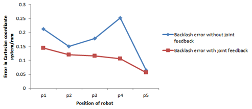
The backlash is generated in the joints of the robot, which is related to the direction of movement of the robot. It can be regarded as an angle error of the joint angle. The position error of the robot in the Cartesian space is generated by the error of each joint, and it can be calculated by the parameter error model of the robot³ when the previous motion state of each joint is known. There are many models that describe the end-effector error of 6R serial robot and they can be separated into two categories: parameter calibration based on model and error model based on sampling. However, both two categories require sampling of robot and the backlash error will exists in sampling points. Figure 1 shows the backlash error of five random points in the Cartesian coordinate system. Those points move in the direction from p1 to p5, and then go back from p5 to p1. At the same time, the laser tracker records each point in different direction of movement and error is calculated by the equation of $\Delta P=\sqrt{\Delta x^2+\Delta y^2+\Delta z^2}$ . The experiment was done 30 times and the error was averaged. In order to make the result contrast, the backlash error is also measured under the condition of the joints feedback. It`s clear that the value of backlash error is far more than the repeated accuracy of 6D serial robot (±0.06mm for KUKA KR210) in some points. The error of the sampling point not only includes the deterministic error caused by the connecting rod parameter but also the random error caused by the backlash and the repeated positioning accuracy of the robot. For the model based sampling, the error measured at one point is not the error when the robot moves to. This is because the robot could be reach one position from different direction. Once the movement direction of joint change, then the backlash error occur. As for the parameter calibration based on kinematic, the sampling point error contains a relatively large random part, and the calculated link parameter error is inaccurate.

Figure 1 Backlash error in Cartesian coordinate system.

This paper eliminates the backlash by installing grating at the first three joints. The backlash error at each joint can be nearly zero by establishing a PID model with the grating feedback. The relationship between the grating readings and the actual rotation angle becomes critical when it is known that raster feedback can accurately reach a joint angle. In fact, due to the existence of the robot geometric parameters error, the actual value of the joint rotation angle of the robot is not necessarily related to the grating reading, which is different in the case of other joint changes. At the same time, only three gratings are installed at robot joints, and it is impossible to calibrate the kinematic parameters of the robot under the condition of joint feedback. Referring to the principle of accuracy compensation, a method of error coupling is proposed in this paper. The spatial position error of the target point is corrected by only rotating the first three axes of the robot. Hence, based on the similarity principle of the space error,⁴ an estimation model of space error of robot is established. The error of the target point can be transformed into the angle error of the first three joints by the error coupling model. And finally, the error is corrected by the closed loop feedback of the first three joint. By means of Kriging interpolation,^5,6 the position error estimation model is established:

$\widehat{e_l}=w^T{e}_l,l=x,y,z$  （1）

 Where $\widehat{e_l}$ is the estimation error of composition point; $w\in R^m$ is the weighted vector between composition point and sampling points; $e_l\in R^m$  represents the vector of the errors of sampling points in the $l$ direction.

 Weighted vector can be obtained by the following formula:

$\{\begin{array}{l}\lambda =(F^T{R}^{-1}F)(F^T{R}^{-1}r-f)\\ W=R^{-1}(r-F\lambda )\end{array}$  （2）

Where $\lambda$ is the Lagrange multiplier, $f={[1{\theta }_1\cdots {\theta }_n]}^T$  ,and $F\in R^m$ denote the angle matrix constructed by each point`s $f$ ; $r\in R^m$ is the correlation vector between composition point and sampling points;$R\in R^{m\times m}$ is the correlation vector between sampling points. The calculated method of correlation between two points based on Gaussian model:

$r_{i,j}=S(\xi ,{\theta }_i,{\theta }_j)={\displaystyle \prod _{k=1}^n\exp (-{\xi }_k\left|{\theta }_{i,k}-{\theta }_{j,k}\right|)}$  （3）

Where ${\xi }_k\in R^n$ denotes the parameter of Gaussian model, which can be obtained by maximum likelihood estimation.

The error coupling model is：

$\Delta X={\left[{\left(\frac{\partial P}{\partial X}\right)}^{\text{T}}\frac{\partial P}{\partial X}\right]}^{-1}{\left(\frac{\partial P}{\partial X}\right)}^{\text{T}}\Delta P$  （4）

Where $\Delta X={[\begin{array}{ccc}\Delta {\theta }_1& \Delta {\theta }_2& \Delta {\theta }_3\end{array}]}^T$  and $\Delta P={[\Delta x,\Delta y,\Delta z]}^T$ .

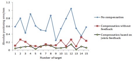
Since the spatial position of the robot is mainly determined by the first three joints, the gratings are only mounted on the first three. The specification of the robot used in this paper is KUKA KR210 extra. Take a 100mm×100mm×100mm grid in the robot operation space, and randomly generate 30 sampling points and 15 test points in this grid. The results of the experiment of the robot are shown in Figure 2. And, the position errors of the robot are obtained under the three conditions no compensation, compensation without feedback and compensation based on joints feedback. As can be seen from the diagram, after eliminating the backlash of the joints by joint feedback, the maximum positioning error of the robot in the test space is 0.14mm, with an average value of 0.078mm. We also have detected that the backlash will lead to a positioning error of 0.1mm~0.25mm in Cartesian space.

Figure 2 Absolute positioning accuracy in three different compensation methods.

Because of the existence of joint backlash, it is impossible to further improve the absolute localization accuracy of the robot by conventional accuracy compensation methods. In this paper, a method of robot accuracy compensation based on joint feedback is proposed. From the preliminary experimental results, the absolute localization accuracy of robot is improved, which demonstrated that this method is effective. The follow-up should verify this method in a larger space and the joints of A4, A5, A6 should be mounted with gratings, since the backlashes of joints A4, A5, A6 still exist.

Author declares that there is none of the conflicts.

References

- Veitschegger WK, Wu CH. Robot calibration and compensation. IEEE Journal on Robotics & Automation. 1988;4(6):643–656.
- Nubiola A, Bonev IA. Absolute calibration of an ABB IRB 1600 robot using a laser tracker. Robotics and Computer–Integrated Manufacturing. 2013;29(1):236–245.
- Wei Z. Theory and Experiment of Industrial Robot Accuracy Compensation Method Based on Spatial Interpolation. Journal of Mechanical Engineering. 2013;49(3):42.
- Bai Y, Cong M, Yang X, Liu D. Kinematic parameter identification for 6R serial robots based on a 6–parameter model. Jiqiren/robot. 2015;37(4):486–492.
- Zeng Y, Tian W, Li D, Wenhe L. An error–similarity–based robot positional accuracy improvement method for a robotic drilling and riveting system. International Journal of Advanced Manufacturing Technology. 2017;88(9–12):2745–2755.
- Lophaven SN, Nielsen HB, Søndergaard J. Aspects of the matlab toolbox DACE. Informatics & Mathematical Modelling Technical University of Denmark. 2002. p. 1–23.
©2017 Liu, et al. This is an open access article distributed under the terms of the,
which
permits unrestricted use, distribution, and build upon your work non-commercially.