In this article, a method for robust Fault Detection and Isolation (FDI) is presented. The scientific interest of this work is use of one tool (Bond Graph) not only for modelling of hybrid system, parametric and measurement uncertainties but also for generation of robust fault indicators and thresholds. For this task, first, the hybrid bond graph (HBG) model is established to model the hybrid system using the controlled junctions. Secondly, all parametric and measurement uncertainties are modeled on the HBG model in derivative causality, from this model and using the causal and structural properties of the bond graph tool, the generation of the fault indicators (residues) and thresholds is done directly, those fault indicators called Generalized Analytical Redundancy Relations (GARRs) are valid at all modes and derived systematically from an HBG model. An application to an hydraulic is used to illustrate this method.

Keywords: hybrid bond graph, fault diagnosis, fault indicators, robust, parameter uncertainties, measurement uncertainties

Current systems engineering, industrial and technical processes are increasingly complex; they include sub-systems of various fields of energy. The Bond Graph (BG) is a multi-physics modeling tool based on analogy and exchange of energy power able to model with a single language, systems, regardless of their physical nature. This modeling aspect has been the subject of several publications.¹⁻³ The BG has been used not only for modeling but also for fault detection and isolation (FDI) of complex systems.⁴⁻⁶ The majority of complexes engineering processes are equipped with sensors, actuators, integrated digital circuits and software. In order to protect the complex engineering systems, safety, reliability, availability and maintenance become important to detect rapidly anomalous behavior of the system after the occurrence of a fault, isolate causes of malfunctions, failures and generate alarms: most complex industrial systems are hybrids. Fault diagnosis for hybrid systems has been the subject of intensive research and several approaches have been developed in the literature for the diagnosis of hybrid systems. In 1994, Mosterman and Biswas⁸ have developed an approach which extends the BG theory,⁷ called Hybrid Bond Graph (HBG) to model the discrete mode changes of hybrid systems, in addition to the junctions of BGs, the HBG methodology uses controlled junctions. In literature, several studies have been proposed⁹⁻¹² based on HBG approach for the diagnosis of hybrid systems. The majority of these works does not address robustness. Ghoshal et al.,¹³ have presented a method for robust diagnosis taking into account parameter uncertainties using pseudo-bond graph to model and diagnosis a hybrid thermo-fluid system, the Linear Fractional Transformation (LFT) form is used to model parameter uncertainties directly on pseudo-bond graph model. The method was tested and the simulations results are given. In the work of Borutzky,¹⁴ a method of robust FDI is presented based on incremental bond graph for hybrid systems, the principle of the method is the generation of thresholds taking into account parameter uncertainties and changes in the discrete mode. An application to a converter circuit to illustrate the method is given. And In,¹⁵ the author, showed that the incremental bond graphs can be used to determine adaptive mode-dependent ARR thresholds in order to obtain robust diagnosis, the bond graph model for hybrid system and mode identification are presented. The method was illustrated by an application on a power electronic system. In,¹⁶ we have developed a method based on HBG-LFT to obtain a robust diagnosis for hybrid systems. The system is modeled using HBG and the parameter uncertainties are modeled graphically using LFT form, the residues and adaptive thresholds are generated from HBG-LFT model. These residues are robust to parameter uncertainties and valid at all modes, the method was tested on a hydraulic hybrid system, and in,¹⁷ we have studied robustness with respect to measurement uncertainties by modeling these uncertainties directly on the HBG model. In the work presented in this manuscript; we will consider both parameter and measurement uncertainties^18,19 for hybrid system modeled by HBG approach to detect defaults. The innovative interest of the present research is essentially based on the use of the HBG tool for first; modeling the discrete mode changes, second; modeling of the parameter and measurement uncertainties graphically, and third; obtain a robust diagnosis by exploiting the causal and structural proprieties, thereby, the systematic generation of robust fault indicators is systematic. The rest of the article is organized as follows: modeling of parameter and measurement uncertainties by bond graph approach is presented in Section 2 and the proposed method for robust diagnosis taking into account parametric and measurement uncertainties based on hybrid bond graph approach in Section 3. Section 4 presents an application on a hydraulic system to validate this method and a conclusion is given in section 5.

Modeling of parametric uncertainties

In order to model parametric uncertainties by bond graph approach, two methods are presented in.¹⁶ In this work, the method used is based on (bond graph- Linear Fractional Transformation BG-LFT) representation. The principle of this method is to replace the BG elements by the corresponding BG-LFT elements to obtain two parts; nominal part and uncertain part. The nominal part is used for calculation of residue, and the uncertain part for the thresholds. Figure 1 shows a BG- R element in the LFT form. An R element in resistance causality with uncertainties can be presented as following Equation (1):

$\{\begin{array}{c}{e}_R=R_n\left(1+{\delta }_R\right).f_R\\ e_R=R_n{f}_R+{\delta }_R.z_R\\ e_R=R_n{f}_R-w_R\\ {\delta }_R=\frac{\Delta R}{R_n}\end{array}$(1)

With: $z_R=R_n.f_R,R_n.{\delta }_R,\Delta R,e_R$and $f_R$are respectively, the nominal value, the multiplicative uncertainty, the additive uncertainty, the effort and the flow variable of R element. $w_R$is a fictive input that represents the effort added by the parameter uncertainty. The LFT form in robust diagnosis has advantages among them:

1. The causality and the structural proprieties of the elements on the nominal model remain unchanged by introducing the uncertainties.
2. The nominal and uncertain parts are separated, and the parameter uncertainties are easily evaluated and explicitly represented in the graphical tool.¹³

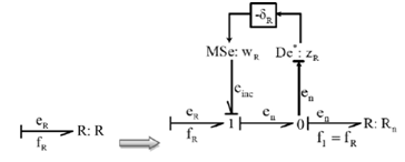
Figure 1 R element in resistance causality using LFT form.

Modeling of measurement uncertainties in a BG context

Mostly, the information provided by sensors are noisy or obtained with a certain precision, therefore, take account of measurements uncertainties is necessary in the diagnostic scheme in order to avoid the problems related to false alarms and no detections. The interest of using this approach based on BG theory for modeling the measurement uncertainties is to use the properties of the tool (BG) to generate residues and thresholds. In BG methodology, the ARRs are considered as residuals. Theoretically, the residues are equal to zero in normal situation, without considering the uncertainties and model errors. The presence of uncertainties on the sensors uncertainties, and if the measurement errors are an additive and bounded error, then, the residual can be bounded by two thresholds. The latter can be obtained using the BG model. Using the BG theory, measurement errors are modeled by replacing the junction containing the detector by its equivalent (Figure 2). The measurement error is replaced by a virtual source of flow (effort) according to the detector De(Df ).¹⁴ Figure 2 shows modeling of measurement uncertainties, the obtained equations are given in Equation (2) and (3).

$\left(a\right)\{\begin{array}{c}{e}_1=SSe\\ e_2=SSe\\ e_3=SSe\end{array}\Rightarrow \left(b\right)\{\begin{array}{c}{e}_1=e_4-{\zeta }_{SSe}=SSe-{\zeta }_{SSe}\\ e_2=e_5-{\zeta }_{SSe}=SSe-{\zeta }_{SSe}\\ e_3=e_6-{\zeta }_{SSe}=SSe-{\zeta }_{SSe}\end{array}$ (2)

$\left(c\right)\{\begin{array}{c}{f}_1=SSf\\ f_2=SSf\\ f3=SSf\end{array}\Rightarrow \left(d\right)\{\begin{array}{c}{f}_1=f_4-{\zeta }_{SSe}=SSf-{\zeta }_{SSf}\\ f_2=f_5-{\zeta }_{SSe}=SSf-{\zeta }_{SSf}\\ f_3=f_6-{\zeta }_{SSe}=SSf-{\zeta }_{SSf}\end{array}$

The following references are given for more details on the modelling of parameter uncertainties^14,16,18,19 for measurements uncertainties, based on BG methodology.

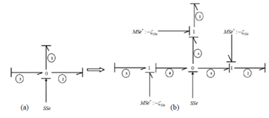
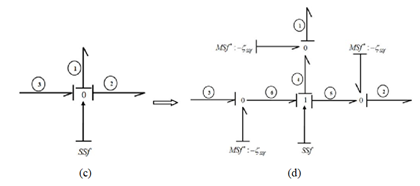
Figure 2 Measurement uncertainly modelling and their equations.

In this section, the proposed method for robust diagnosis based on the HBG approach with controlled junctions and modeling of parametric and measurement uncertainties by BG methodology is presented. The steps of the method are:

1. The hybrid system is modeled by HBG approach using controlled junctions taking account discrete mode changes; The HBG model of the system is obtained.
2. The Diagnostic hybrid bond graph model (DHBG) is obtained by applying the sequential causality assignment procedure for hybrid system diagnosis (SCAPHD).²⁰ The SCAPHD represents the extension of the SCAP by affecting the causality of controlled junction according to the concept of the preferred causality of these controlled junctions.
3. The measurement uncertainties are modeled directly on the DHBG model
4. The parametric uncertainties are represented graphically.
5. For each detector whose causality is reversed,²¹ a robust global candidate residue is generated at this junction.
6. Using the causal and structural proprieties of the HBG tool, the unknown variables are eliminated by covering the causal paths from unknown variables to known (sensors and sources).²²

The objective of this part is to show the proposed method on a hydraulic system: the hybrid system is modeled by hybrid bond graph (HBG) approach with controlled junctions, the DHBG model is obtained by attributing derived causality on the HBG model, then; the parametric and measurement uncertainties are modeled on the obtained DHBG model, the generation of fault indicators is established, residues and thresholds, simulation tests are given to show the residuals with and without defaults. In the following, these steps are detailed. The proposed method is applied to a hybrid hydraulic system shown in Figure 3: The generation of Robust Global Analytical Redundancy Relations (GARRs) with respect to parametric and output (measurements) uncertainties is presented.

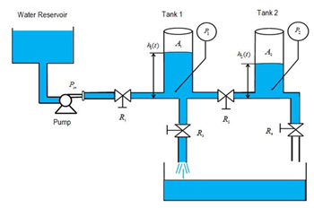
Figure 3 The hybrid Two-Tank system.

First step: Modeling of the hybrid system: the system is composed of two tanks, regulated centrifugal pump modeled as a source of pressure p_in(t) [Pa] and four valves represented by R₁, R₂, R₃ and R₄. A₁[m²] and A₂[m²] are the cross-section areas of the two tanks. The system contains two pressure sensors (p₁(t) and p₂(t)) to measure the pressure at the button of tank A₁ and tank A₂ , respectively; this pressure is proportional to the liquid level, according to:

$P_i(t)=\rho g{h}_t\left(t\right),i=1,2$(4)

Whereis the density of liquid, [kg/m³]; g is the acceleration due to gravity , [m/s²], h_i (t) is liquid height in the tank, [m].

Each valve has two states ON and OFF. The valves’ dynamics is given by:

$f_j\left(t\right)=0,j=1,2,3,4$when the valve is closed

$f_j\left(t\right)=\frac{sign\left(\Delta P\left(t\right)\right).\sqrt{\Delta P\left(t\right)}}{R_j}=C{d}_j.sign\left(\Delta P\left(t\right)\right).\sqrt{\Delta P\left(t\right)}$(5)

When the valve is opened. Where $f_j$the liquid-flow through the valve, [m³/s]; $\Delta p\left(t\right)$is the pressure difference across the valve , [Pa] and $C{d}_j$is the coefficients of discharge,.

In the HBG model of Figure 4; the two tanks are modeled by two storage components with coefficients $C_i=\frac{A_i}{g};i=1,2$The valves are modeled by a set of resistor with parameter ; $R_j=\frac{1}{C{d}_j}$j=1,2,3,4, and controlled-junction with boolean variable $a_{cj}$j =1,2,3,4, representing the state of controlled junctions.

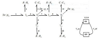
Figure 4 The two-tank acausaled HBG and the finite state automaton of controlled junctions.

Second step: The DHBG (Figure 5) is obtained by affecting all controlled junctions by their preferred causalities, to do this:

1. The output variables of the controlled junctions 1_c3,1_c2 and 1_c4 are assigned as inputs of R₃ , R₂ and R₄ respectively because these junctions have no source adjacently connected to them.
2. The output of 1_c1 is assigned as input variable of 1-port component R₁ since the source Se is connected to1_c1.
3. The source Se and the storage components C₁, C₂ are assigned in preferred derivative causality and the sensor is reversed (dualized).

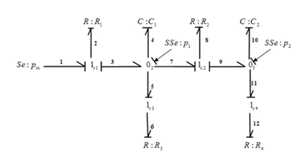
Figure 5 The two-tank DHBG.

Third step: The parameter and measurements uncertainties are graphically modeled on the DHBG model. The Figure 6 shows this representation of uncertainties. Two GARRs can be derived from the model of Figure 6;

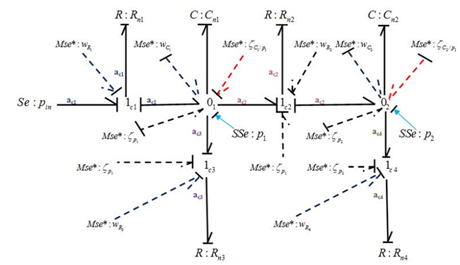
Figure 6 The model of the two tank system in preferred derivative causality with measurement and parameter uncertainties.

The first candidate GARR is

$$GAR{R}_1=a_{c1}.C{d}_1.\left[sign\left(P_{in}-P_1\right)\sqrt{\left|\left(P_{in}-P_1\right)\right|}\right]-C_1.\frac{d}{dt}{P}_1-a_{c2.C{d}_2.\left[sign\left(P_1-P_2\right)\sqrt{\left|\left(P_1-P_2\right)\right|}\right]}.\left(P_1-{\zeta }_{P_1}\right)-a_{c3}.C{d}_3.\sqrt{P_1}\left(P_1-{\zeta }_{P_1}\right)+w_{c1}+w_{\raisebox{1ex}{$c1$}\!\left/ \!\raisebox{-1ex}{$P1$}\right.}$$

And the second candidate GlobalARR:

$GAR{R}_2=a_{c2}.C{d}_2.\left[sign\left(P_1-P_2\right)\sqrt{\left|\left(P_1-P_2\right)\right|}\right].\left(P_1-{\zeta }_{P_1}\right)-C_2.\frac{d}{dt}{P}_2-a_{c4.C{d}_4.}\sqrt{P_2}\left(P_2-{\zeta }_{P_2}\right)+w_{c2}+w_{\raisebox{1ex}{$c2$}\!\left/ \!\raisebox{-1ex}{$P2$}\right.}$

And the second candidate GlobalARR:

These GARRs can be decomposed in two separate parts; the first nominal, called residue and the second uncertain used to calculate the thresholds.

with: $a_{cj}\in \left\{0,1\right\}$are discrete variables representing the state of controlled junction 1_cj

for $j\in \left\{1,2,3,4\right\},{\xi }_{p1},{\xi }_{p2}$are respectively the measurement errors on the first pressure sensor p₁ and on the second pressure sensor p₂ , These measurement errors are bounded as follows: and the virtual inputs of measurement uncertainties .

$\left|{\xi }_{p1}\right|\le {\Delta }_{p1}$, $\left|{\xi }_{p2}\right|\le {\Delta }_{p2}$Where: $w_{c1},w_{c2}$and $w_{\raisebox{1ex}{$c1$}\!\left/ \!\raisebox{-1ex}{$P1$}\right.},w_{\raisebox{1ex}{$c2$}\!\left/ \!\raisebox{-1ex}{$P2$}\right.}$ are respectively the fictitious inputs of parameter uncertainties and the virtual inputs of measurement uncertainties, ${\delta }_{c_1},{\delta }_{c_2}$are the multiplicative uncertainties on the two storage components C ₁,C ₂ and fixed as 5% and ${\xi }_{p1}$,${\xi }_{p2}$ are respectively the measurement errors on the first pressure sensor p₁ and on the second pressure sensor p₂, then errors measures are added to the exact values of the measures of the system. The results presented below show the residues in presence of parameter and output (measurements) uncertainties in normal and faulty operation. The nominal values of parameters used in the simulations of the model are shown in Table 1. Different scenario of simulations was performed to test the effectiveness of the proposed method.

First scenario

Test1: Normal operation (without default), the valves 1 and 2 are open at t=1s, the valves 3 and 4 are closed. The states of the four valves are shown in Figure 7. The residues r₁, r₂ in presence of parametric and measurement uncertainties without default are presented in Figure 8: we note that the residues are equal to zero and do not leave the thresholds. The mode change is observed at t=1s.

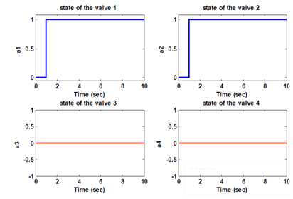
Figure 7 The states of the four valves.

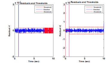
Figure 8 The residues without default.

Test2: Figure 9 shows the residues in normal operation and the valves 1 and valve 2 are open, and the valves 3 and the valve 4 are closed. The states of the valves are presented in Figure 10.

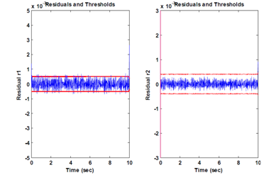
Figure 9 The residues without default.

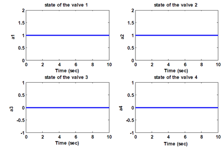
Figure 10 The states of the four valves.

Second scenario

Test1: Faulty operation (with default), the four valves are open. The states of the four valves are shown in Figure 11. A default of 0.2 [Pa] on the first sensor p₁ is occurred between t=2s and t=4s, the responses of residues are shown in Figure 12 & Figure 13 shows the outputs of the system. We note that the default is detected by the two residues. These residues exceed the thresholds during the presence of default.

Test2: Now the default is considered with the following operation; the mode change is at t= 1s. The operation of the system in different states of the valves (opening of the valve 1 and 2 at t = 1s, the valve 3 open and the valve 4 is closed). The sensors are in Figure 14, the states of the valves are in Figure 15. The reaction of residues is shown in Figure 16. In this test, at t = 1s the mode change at t = 1s and detection of default at t = 2s and 4s.

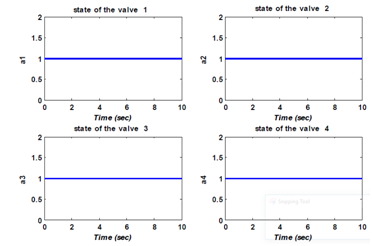
Figure 11 The states of the four valves.

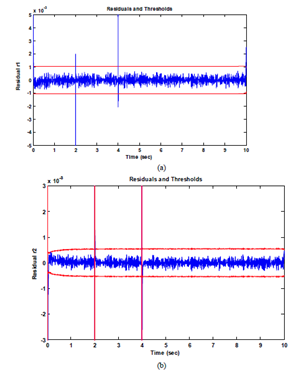
Figure 12 The responses of residues.

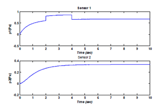
Figure 13 The outputs of the system.

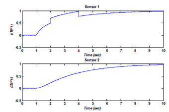
Figure 14 The outputs of the system.

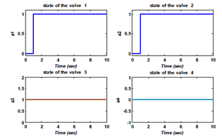
Figure 15 The states of the four valves.

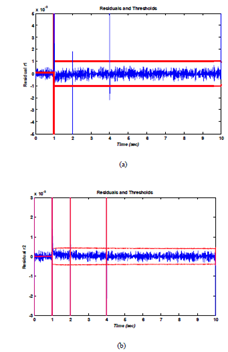
Figure 16 The responses of residues r1, r2.

Test3: Figure 17, 18, 19 show the results of this test. In this case, the default is occurredat t= 1s and t=6s (Figure 17) and the mode change at = 2s (Figure 18). The residues r₁, r₂ are equal to zero and different when the fault is occurred. We note that the two residues are sensitive to the sensor default exceeding the thresholds, thus, generating a false alarm. We can say that the fault has been detected by these two residues r₁, r₂ (Figure 19).

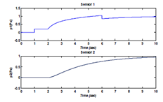
Figure 17 The sensors.

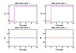
Figure 18 The stats of the valves.

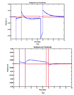
Figure 19 The responses of residues r1, r2.

In this article, a method for robust diagnosis is presented. The interest of this method is the use only one tool (hybrid bond graph) not only for modeling of the discrete mode changes of the hybrid system, and modeling of parametric and measurement uncertainties but also for robust diagnosis. The diagnostic system allows detection of fault on the sensors in the presence of parametric and measurement uncertainties, where uncertainties are modeled directly on the hybrid bond graph model. The causal and structural proprieties are used for generation of residues and thresholds. The residues are called GARRs; are generated directly from a diagnostic hybrid bond graph model, robust to parametric and measurement uncertainties, and describe the system at different modes by using different corresponding value of acj. The results presented in this article show the effectiveness of the diagnostic method in terms of detecting defaults on the sensors using bond graph methodology.

None

The author declares there is no conflict of interest.

1. Ould Bouamama B, Samantaray AK, Staroswiecki M. Derivation of constraint relations from bond graph models for fault detection and isolation. Simulation Series. 2003;35:104–109.
2. Ould Bouamama B, Samantaray AK, Medjaher K, et al. Model builder using functional and bond graph tools for FDI design. Control Engineering Practice. 2005;13(7):875 –891.
3. Samantaray A K, Medjaher K, Ould Bouamama B, et al. Component based modelling of thermo-fluid systems for sensor placement and fault detection. Simulation. 2004;80:381–398.
4. Karnopp D, Margolis DL, Rosenberg RC. Systems dynamics: modeling and simulation of mechatronic systems. 2nd ed. New York: A Wiley-Interscience Publication; 2006.
5. Mosterman PJ, Biswas G. Behavior generation using model switching: A hybrid bond graph modeling technique. Trans Soc Simul. 1994;27:177–182.
6. Low CB, Wang D, Arogeti S, et al. Causality assignment and model approximation for hybrid bond graph: Fault diagnosis perspectives. IEEE Transactions on Automation Science and Engineering. 2010;7(3):570–580.
7. Low CB, Wang D, Arogeti SA, et al. Fault parameter estimation for hybrid systems using hybrid bond graph. Proceedings of the Control Applications, (CCA) Intelligent Control, (ISIC), IEEE; 2009 July 8–10, 2009:1338–1343.
8. Daigle MJ, Koutsoukos XD, Biswas G. An event-based approach to integrated parametric and discrete fault diagnosis in hybrid systems. Transactions of the Institute of Measurement and Control. 2010;32:487–510.
9. Arogeti SA, Wang D, Low CB, et al. Fault detection isolation and estimation in a vehicle steering system. IEEE Transactions on Industrial Electronics. 2012;59(12):4810–4820.
10. Ghoshal SK, Samanta S, Samantaray AK. Robust Fault Detction and Isolation of Hybrid Systems with Uncertain Parameters. Journal of Systems and Control Engineering. 2012;226(8):1013–1028.
11. Borutzky W. Fault indicators adaptative thresholds from hybrid system models. Proceedings of the 7th Vienna International Conference on Mathematical Modelling; Austria. Vienna University of Technology; 2012. p. 392–397.
12. Rahal MI, Ould Bouamama B, Meghebbar A. Hybrid Bond Graph for Robust Diagnosis–Application to Hydraulic System, Proceedings of the 3rd IEEE International Conference on Systems and Control, (ICSC’13), Algiers; 2013 Oct 29–31; Algeria. p. 1080–1085.
13. Djeziri MA, Ould-Bouamama B, Merzouki R.Modelling and robust FDI of steam generator using uncertain bond graph model. J Process Control. 2009;19(1):149–162 .
14. Touati Y, Merzouki R, Ould Bouamama B. Fault detection and isolation in presence of input and output uncertainties using bond graph approach. Proceedings of the IMAACA; 2011. p. 221–227.
15. Dauphin-Tanguy G, Rahmani A, Sueur C. Bond graph aided design of controlled systems. Simulation Practice and theory. 1999;7(5-6):493–513.
16. Kam CS, Dauphin-Tanguy G. Bond graph models of structured parameter uncertainties. Journal of the Franklin Institute. 2005;342(4):379–399.
17. Rahal MI, Ould Bouamama B, Meghebbar A. Hybrid Bond Graph for robust diagnosis to measurement uncertainties. Proceedings of the 5th IEEE International Conference on Systems and Control, (ICSC’16); 2016 25-27 May. Marrakech, Morocco. 2016. p. 439–444.
18. Djeziri MA. Diagnostic des Systèmes Incertains par l’Approche Bond Graph, [dissertation]. Lille university, France; 2007.
19. Touati Y, Merzouki R, Ould Bouamama B. Robust diagnosis to measurement uncertainties using bond graph approach: Application to intelligent autonomous vehicle. Mechatronics. 2012;22(8):1148–1160.
20. Wang D, Yu M, Low C. B, et al. Model-based health monitoring of hybrid systems. New York: Springer; 2013.
21. Ould Boumama B. Diagnostic en ligne à base de modèle Bond graph. REE Revue de l’Electricité et de l’Electronique. 2010;(2):111–117.
22. Merzouki R, Kumar Samantaray A, Mani Pathak P, et al. Intelligent mechatronic systems: modeling, control and diagnosis. London: Springer; 2013.
23. Borutzky W. Bond Graph model-based system mode identification and mode dependent fault thresholds for hybrid systems. Mathematical and computer modeling of Dynamical systems. 2014;20(6):584–615.
24. Ould bouamama B, Dauphin-Tanguy G. Modélisation par bond graph: Éléments de base pour l'énergétique. Techniques de l'ingénieur. Génie énergétique. 2006(BE8280).
25. Marquid-Favre W, Jardin A. Bond Graph pour la concetption des systemes mecatroniques. Techniques de l'ingénieur. 2012.