The wheeled mobile robot with differential thrust consists of two independent active wheels and a passive spherical wheel. Assuming its net rolling and non-uncertainty, this robot is a nonlinear system bound to non-holonomic constraints. This system also falls into the category of systems with a lack of operators. Tracing time travel paths is one of the most difficult issues in the field of wheeled robots that we will address in this article. In this regard, first the kinematic model of the system with the presence of uncertainty on the control inputs is expressed in which the linear velocity and angular velocity of the robot are considered system inputs. After determining the desired reference paths, using the linearization of the designed feedback controller ensures the stability of all system state variables globally. The controller is then designed with adaptive rules to solve the problem of tracking time paths based on input-output control in the presence of uncertainties. The stability of this controller is also proven globally. Finally, the performance of the designed controllers to compensate for the uncertainties will be compared by comparing the results.

Keywords: asymptotic stability, feedback linearization, mobile robots, uncertainty, nonholonomic systems, tracking control

In recent years, mobile basic robots have found a special place in various industries and consequently have been considered by many researchers.¹ Depending on the environment in which they are used, these robots use movement tools appropriate to that environment.² The wheel is the most widely used drive mechanism due to its simplicity, acceptable speed and high efficiency. Wheeled robots are a group of mobile robots that have a variety of applications in various industries, especially in hazardous environments such as space, war and the movement of sensitive cargo and contaminated waste. In the article,³ suitable and suitable for different types of kinematic and dynamic wheeled robots. These robots will be bound to non-holonomic constraints if they roll smoothly and in the absence of uncertainty.⁴ The guidance of wheeled robots is divided into two issues: motion planning and control. Plans the movement of the robot's path so that it meets the operational objectives and the control moves the robot on the designed path. Wheeled robots are very non-linear and are classified in the group of systems with a lack of operators.⁵ These robots also have a non-quadratic multi-input-multi-output system, which has made the problem of controlling these robots in full state mode a challenging problem. In controlling wheeled robots, three main issues are widely raised. Stabilization around optimal positions, trajectory in Cartesian space and trajectory of time travel paths, among which the pursuit of time trajectories has received more attention of researchers.⁶

Linearization of feedback a nonlinear system has many applications in controlling nonlinear systems and processes. This method has appeared in powerful and efficient control of nonlinear systems and has significant capabilities.⁷ In this dissertation, first, this method is briefly introduced and its advantages and disadvantages are also discussed. Among the limitations of this method:

1. Proper performance in a specific part of nonlinear systems
2. Need to access all system mode variables
3. Low resistance against uncertainties.

The first limitation is that the use of this method requires the fulfillment of conditions such as existence of a certain relative degree and the minimum phase of the system.⁸ The second and third limitations also indicate the need for this method to have an accurate model of the system in order to eliminate nonlinear parts and achieve a completely linear form.⁹ In line with the third case, it should be noted that in the presence of uncertainties, this method leads to an inaccurate linearization and thus reduces the stability and efficiency of the system.¹⁰

Linearization with feedback is a method of designing nonlinear controllers that has attracted much interest from researchers in recent years. However, in real applications as a result of the implementation of such control algorithms due to the limitations of this method and its computational needs are less seen. Among other things, in this algorithm, all the modes of the system must be available and usually the system is not guaranteed against uncertainty.¹¹ Therefore, a lot of research has been done to overcome the problem of uncertainty (parametric) by external ring design techniques and retrofit control designs.¹²

The method of linearization method with feedback is based on the idea of transferring nonlinear dynamics to a linear form using state-of-the-art feedback, which includes two modes of input-mode linearization (which leads to complete system linearization) and input-output linearization. (Which only leads to the linearization of part of the nonlinear system).¹³ As mentioned, the main problem of this method in the above two cases is the need to have a completely accurate model of the system to eliminate the effect of nonlinear parts completely,¹⁴ which is important despite the uncertainties in the system model. There are two types of uncertainty in control systems: a) parametric uncertainty,¹⁵ b) modeling uncertainty (unmodulated dynamics and environmental factors affecting the system).¹⁶

There are always differences between the identified model and the actual system. This discrepancy can be due to several reasons. Including:

1. Simplifying the dynamics of a very complex system
2. Lack of sufficient knowledge of physical laws
3. Complete ignorance of system dynamics parameters
4. 4-Complexity of system identification algorithms (nonlinearity optimization).
5. Approximation of nonlinear systems with a linear system.

In order to achieve the desired control goals, what we know (identified system model) must be more than what we do not know.

Given the above, the purpose of robust control:

"Design is a controller that achieves all design goals despite the uncertainties in the system."

Robust control methods in eliminating the effect of perturbation, exposure to parameters with rapid changes and reducing the effect of parametric uncertainties and unmodulated system dynamics can well help the linearization method with feedback.¹⁷

Some of the control algorithms have been based on linearization. In order to linearize a nonlinear system, it is possible to find a linear approximation of the main process around a work point or common practice. For nonlinear systems, it is a traditional linear modeling method that uses Taylor¹⁸ expansion of the system function and, regardless of the order of 2 or higher sentences, the system equations are converted to linear equations, and then the design of the controller is carried out using linear system theory. But this method could create limitations, especially for nonlinear systems. Therefore, it is essential that effective control methods be performed for nonlinear systems. Since 1980, many control methods have been presented for nonlinear systems, including linearization with feedback based on differential equations of the system that have a wide application in nonlinear systems.¹⁹

Linearization with feedback is also an effective way of designing a controller for a nonlinear system because a nonlinear system is transformed into a linear system using a homomorphic transform and state feedback.²⁰ But pure state feedbacks due to Brockett necessary condition cannot be used in order to control the nonholonomic system. Therefore the dynamic feedback linearization method has been used in order to control the WMRs as a nonholonomic system.

According to the above, in the continuation of this article, in order to strengthen the linearization method with feedback against parametric uncertainties, using the method of estimating uncertainties using the estimation method that the desired values The kinematics of the system is obtained, causing a resistor to be added to the linear controller with feedback, so that the nonlinear system is able to follow the reference path optimally in the range of parameter changes from minimum to maximum values. . The advantages of such a combination are the reduction of the effect of parametric uncertainties, the tendency of the chase error to zero in the presence of uncertainties, the reduction of the interference effect and the increase of the system resistance to external disturbances compared to the conventional linear controller. Therefore, it can be claimed that by using this method, the existing problems in linearization with feedback, which were mentioned at the beginning, have been somehow solved.

In this paper, the main purpose of designing a kinematic controller in the presence of uncertainties in the inputs of the tractor-trailer system is to follow the time path of reference paths. To achieve this, feedback linearization control methods have been used so that the kinematic controllers produce the required speeds and a dynamic controller using the left and right wheel torques, the required control speeds. Provides cinematic actors.

In this paper, after the introduction of robotic kinematics, using the intrinsic capacity of the regression controller in controlling systems with operator deficiency, a linear feedback controller in Cartesian space has been designed that ensures the stability of all mode variables without limitation in the field of absorption. Slowly the controller is then designed for input-output. This controller guarantees the stability of the output and the constraint of all mode variables, as well as the design capacity for the controller resistant to finite uncertainties. A controller feedback is then proposed for this robot using linearization method. This controller also guarantees the stability of all mode variables, but is valid to the extent that the variables changed are uniquely reversible. The simulation results are then presented to evaluate the performance of the proposed controllers under ideal conditions as well as in the presence of perturbations. Finally, we summarize and conclude this research.

The considered wheeled robot as shown in Figure 1 is a tractor towing a trailer. The main discussion in the study of these robots is the existence of nonholonomic constraints in the kinematics of these systems. In Figure 2, a WMR with a trailer is shown. The tractor is equipped with two driving wheels and a spherical wheel is used for stable motion, while the trailer has two passive wheels. Tractor and trailer are connected to each other via a revolute joint in point P that is located in the middle of the driving wheels. Here, it is assumed that the mobile robot wheels has non-uncertainty condition in the lateral direction and as a disk has a single point of contact with the surface of the movement. A coordinate system (X ,Y) is considered as the inertial frame. d denotes the distance between points P₀ and P₁, and points P_c and Q_c represent the tractor and trailer centroids.²¹

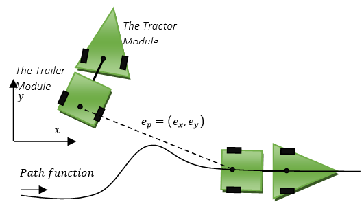
Figure 1 Trajectory following for a WMR.

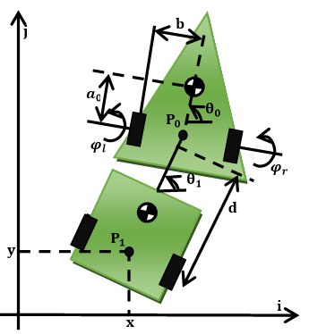
Figure 2 Tractor-trailer wheeled robot.

System constraints can be written in matrix form as follows

$A(q)\dot{q}=\left(\begin{array}{cccc}\sin {\theta }_0& -\cos {\theta }_0& 0& -d\cos ({\theta }_0-{\theta }_1)\\ \sin {\theta }_1& -\cos {\theta }_1& 0& 0\end{array}\right)=0$   (1)

where $q={(x,y,{\theta }_0,{\theta }_1)}^T$ is system configuration vector. (x,y) is the coordinate of point P₁ in the inertial frame, θ₀ and θ₁ represent the orientation of the tractor and trailer with respect to the inertial frame, respectively. Also, A(q) is system constraint matrix.

Kinematic equations of the mobile robot can be written as

$\dot{q}(t)=S(q)u$   (2)

where $u={(u_1,u_2)}^T$ describes an independent set of variables which is here the system input vector. u₁ is the linear velocity of point Q and u₂ is angular velocity of the tractor.

Also S(q) matrix can be found as

$S(q)=\left(\begin{array}{cc}\cos {\theta }_1& 0\\ \sin {\theta }_1& 0\\ 0& 1\\ \frac{1}{d}\tan ({\theta }_0-{\theta }_1)& 0\end{array}\right)$   (3)

Moreover we can write the following condition

$S^T(q)A^T(q)=0$   (4)

Generation of reference trajectories

From equations (2) to (4) reference variables can be calculated as

$\{\begin{array}{c}{\theta }_{1r}(t)=ATAN2\left\{{\dot{y}}_r(t),{\dot{x}}_r(t)\right\}\\ {\theta }_{0r}(t)={\theta }_{1r}+a\tan \left(\frac{d{\dot{\theta }}_{1r}}{u_{1r}}\right)\end{array}$   (5)

where ATAN2 is the four-quadrant inverse tangent function.

Reference inputs will be as follow

$\{\begin{array}{c}{u}_{1r}(t)=\pm \sqrt{{\dot{x}}_r^2(t)+{\dot{y}}_r^2(t)}\\ u_{2r}(t)={\dot{\theta }}_{1r}+d{u}_{1r}\frac{\left({\stackrel{⃛}{y}}_r{\dot{x}}_r-{\stackrel{⃛}{x}}_r{\dot{y}}_r\right)u_{1r}^2-3\left({\ddot{y}}_r{\dot{x}}_r-{\ddot{x}}_r{\dot{y}}_r\right)\left({\dot{x}}_r{\ddot{x}}_r+{\dot{y}}_r\right)}{u_{1r}^6+d_2{\left({\ddot{y}}_r{\dot{x}}_r-{\ddot{x}}_r{\dot{y}}_r\right)}^2}\\ \end{array}$   (6)

It is assumed that reference trajectories $x_r(t)$ , $y_r(t)$ , ${\theta }_{0r}(t)$  and ${\theta }_{1r}(t)$ and reference velocity inputs and their derivatives are continuous and uniformly bounded. 

Assume that in this order of derivation we get the direct relation between y and u on the system as follows:

$y^{(n)}=f_1+a(x)u$   (7)

In this case, we act as follows

$y^{(n)}=y_d^{(n)}+e^{(n)}=v$   (8a)

$v=y_d^{(n)}-k_{1}e-k_1\dot{e}\mathrm{....}-k_n{e}^{(n-1)}$   (8b)

$f_1+a\left(x\right)u=v$   (8c)

$u=\frac{1}{a(x)}\left(v-f_1\right)$   (8d)

$k_{1}e+k_1\dot{e}\mathrm{....}+k_n{e}^{(n-1)}+e^{(n)}=0$   (8e)

As can be observed according to equation (8b), we first create v and then from (8c), we can obtain u and thus our control input is obtained. According to the equation (8e) with the right choice of the coefficients, we can take the poles of the error dynamics to any place where we want, and thus we can stabilize the error around the origin. In these equations, f₁ is obtained from system states.

Dynamic feedback linearization for the tractor-trailer with uncertainty 

In this section a dynamic feedback linearization method is proposed for the tractor-trailer system in order to steer the WMR asymptotically follow reference trajectories. In another words control law u should be designed so that the tractor-trailer system from any arbitrary initial condition for the system from the acceptable Cartesian space (Ω), asymptotically follow reference trajectories. In this method, we must first obtain a direct relationship between the input and output of the system. This can be performed differentiating from y as the output array of the system. Therefore by differentiating from y a direct relation between u and y is obtained. Subsequently control law u is designed in order to eliminate the effect of the nonlinear parts and also to obtain v in order to stabilize the error dynamics.

For the given system, the kinematic equations are defined according (2) and (3) as follows

$\{\begin{array}{c}\dot{x}=\left(u_1+{\delta }_1\right)\cos {\theta }_1\\ \dot{y}=\left(u_1+{\delta }_1\right)\sin {\theta }_1\\ {\dot{\theta }}_0=\left(u_2+{\delta }_1\right)\\ {\dot{\theta }}_1=\frac{\left(u_1+{\delta }_1\right)}{d}\tan \left({\theta }_0-{\theta }_1\right)\end{array}$   (9)

Now differentiating from $\dot{x}$ and $\dot{y}$ yields

$\{\begin{array}{c}\ddot{x}={\dot{u}}_1\cos {\theta }_1-\frac{{\left(u_1+{\delta }_1\right)}^2}{d}\sin {\theta }_1\tan \left({\theta }_0-{\theta }_1\right)\\ \ddot{y}={\dot{u}}_1\sin {\theta }_1-\frac{{\left(u_1+{\delta }_1\right)}^2}{d}\cos {\theta }_1\tan \left({\theta }_0-{\theta }_1\right)\end{array}$   (10)

Continuing this process we will have

$\ddot{x}={\ddot{u}}_1\cos {\theta }_1-\frac{2{\dot{u}}_1\left(u_1+{\delta }_1\right)}{d}\sin {\theta }_1\tan \left({\theta }_0-{\theta }_1\right)-\left[\frac{{\left(u_1+{\delta }_1\right)}^2}{d}\sin {\theta }_1\left(1+{\tan }^2\left({\theta }_0-{\theta }_1\right)\right)\times \left(u_2+{\delta }_2-\frac{\left(u_1+{\delta }_1\right)}{d}\tan \left({\theta }_0-{\theta }_1\right)\right)\right]-\frac{{\left(u_1+{\delta }_1\right)}^3}{d^2}{\tan }^2\left({\theta }_0-{\theta }_1\right)\cos {\theta }_1$   (11)

And

$\ddot{y}={\ddot{u}}_1\sin {\theta }_1+\frac{2{\dot{u}}_1\left(u_1+{\delta }_1\right)}{d}\cos {\theta }_1\tan \left({\theta }_0-{\theta }_1\right)+\left[\frac{{\left(u_1+{\delta }_1\right)}^2}{d}\cos {\theta }_1\left(1+{\tan }^2\left({\theta }_0-{\theta }_1\right)\right)\times \left(u_2+{\delta }_2-\frac{\left(u_1+{\delta }_1\right)}{d}\tan \left({\theta }_0-{\theta }_1\right)\right)\right]-\frac{{\left(u_1+{\delta }_1\right)}^3}{d^2}{\tan }^2\left({\theta }_0-{\theta }_1\right)\sin {\theta }_1$   (12)

As can be seen, direct relation between the outputs and the inputs of the system has been established and equations (11) and (12) can be expressed in the matrix form as follows

$\stackrel{⃛}{X}=JU+A$   (13)

where, $U=\left[\begin{array}{c}{\ddot{u}}_1\\ u_2\end{array}\right],A=\left[\begin{array}{c}{A}_1\\ A_2\end{array}\right]and\stackrel{⃛}{X}=\left(\begin{array}{c}\stackrel{⃛}{x}\\ \stackrel{⃛}{y}\end{array}\right)$ are given as follows

$\left[\begin{array}{c}\stackrel{⃛}{x}\\ \stackrel{⃛}{y}\end{array}\right]=\left[\begin{array}{c}\cos {\theta }_1\frac{{\left(u_1+{\delta }_1\right)}^2}{d}\sin {\theta }_1\left(1+{\tan }^2\left({\theta }_0-{\theta }_1\right)\right)\\ \sin {\theta }_1\frac{{\left(u_1+{\delta }_1\right)}^2}{d}\cos {\theta }_1\left(1+{\tan }^2\left({\theta }_0-{\theta }_1\right)\right)\end{array}\right]\left[\begin{array}{c}{\ddot{u}}_1\\ u_2+{\delta }_2\end{array}\right]$   (14)

$J=\left[\begin{array}{cc}\cos {\theta }_1& -\frac{{\left(u_1+{\delta }_1\right)}^2}{d}\sin {\theta }_1\left(1+{\tan }^2\left({\theta }_0-{\theta }_1\right)\right)\\ \sin {\theta }_1& \frac{{\left(u_1+{\delta }_1\right)}^2}{d}\cos {\theta }_1\left(1+{\tan }^2\left({\theta }_0-{\theta }_1\right)\right)\end{array}\right]$   (15)

$A_1=-\frac{2\left(u_1+{\delta }_1\right){\dot{u}}_1}{d}\sin {\theta }_1\tan \left({\theta }_0-{\theta }_1\right)-\frac{{\left(u_1+{\delta }_1\right)}^2}{d}\sin {\theta }_1\left(u_2+{\delta }_2-\frac{\left(u_1+{\delta }_1\right)}{d}\tan \left({\theta }_0-{\theta }_1\right)\left(1+{\tan }^2\left({\theta }_0-{\theta }_1\right)\right)\right)-\frac{{\left(u_1+{\delta }_1\right)}^2}{d^2}{\tan }^2\left({\theta }_0-{\theta }_1\right)\cos {\theta }_1$   (16)

$A_2=-\frac{2\left(u_1+{\delta }_1\right){\dot{u}}_1}{d}\sin {\theta }_1\tan \left({\theta }_0-{\theta }_1\right)-\frac{{\left(u_1+{\delta }_1\right)}^2}{d}\sin {\theta }_1\left(u_2+{\delta }_2-\frac{\left(u_1+{\delta }_1\right)}{d}\tan \left({\theta }_0-{\theta }_1\right)\left(1+{\tan }^2\left({\theta }_0-{\theta }_1\right)\right)\right)$   (17)

Since the relative degree is equal to the order of the derivatives after the direct relation between inputs and outputs, therefore the relative degree is equal to 3. In the dynamic feedback linearization method, the syetem input array should be obtained in such a way that the state equations of the system are converted into linear form, and then u is determined in order to stabilize the system.

Now consider the system error as

$E=X-X_r$   (18)

Assuming u as follows to stabilize the system

$\left[\begin{array}{c}{\ddot{u}}_1\\ u_2+{\delta }_2\end{array}\right]=J^{-1}\left(-A+{\stackrel{⃛}{X}}_r-k_1\stackrel{⃛}{E}-k_2\dot{E}-k_{3}E-k_4{\displaystyle \int Edt}\right)$   (19)

The inverse of the matrix J is also as follows

$J^{-1}=\frac{1}{\frac{{\left(u_1+{\delta }_1\right)}^2}{d}\left(1+{\tan }^2\left({\theta }_0-{\theta }_1\right)\right)}\times |\begin{array}{cc}\begin{array}{cc}\cos {\theta }_1\left(\frac{{\left(u_1+{\delta }_1\right)}^2}{d}1+{\tan }^2\left({\theta }_0-{\theta }_1\right)\right)& \frac{{\left(u_1+{\delta }_1\right)}^2}{d}\sin {\theta }_1\left(1+{\tan }^2\left({\theta }_0-{\theta }_1\right)\right)\\ -\sin {\theta }_1& \cos {\theta }_1\end{array}& \end{array}$   (20)

After substituting the equation of (20) in (19), the system error dynamics is calculated as follows

$\stackrel{⃛}{E}+k_1\stackrel{⃛}{E}+k_2\dot{E}+k_{3}E-k_4{\displaystyle \int Edt}=0$   (21)

In the above relation k₁, k₂, k₃ and k₄ are control gains. These control gains should be positive for the stability of the system. Also according to the Roth stability method, condition $k_2>\frac{k_3}{k_1}$ must be satisfied for the complete stability of the system and the convergence of the system errors to the point of equilibrium at the origin. Therefore it can be concluded that

$E\to 0\to \{\begin{array}{c}x\to x_r\\ y\to yr\end{array}$   (22)

Therefore the stability of the system around reference trajectories is guaranteed.

In this section, the obtained results from applying the dynamic feedback linearization control law proposed in the previous section to track the reference trajectories to evaluate its performance. In Table 1, the values of the control parameters used in control algorithm have been presented.

To estimate the uncertainties as a source of uncertainties exist for TTWMR, we can assume that the generalized coordinates of the system (q) can be measured with a specific time interval using measuring systems (for example, a vision system). With this assumption, one of the simplest methods for estimating the uncertainty values is using a priori knowledge of the system which contains the data from previous time steps. In this regard, taking into account the kinematic equation of the system from Error! Reference source not found., we can estimate the uncertainty vector $\widehat{\delta }={\left[\begin{array}{cc}{\widehat{\delta }}_1& {\widehat{\delta }}_2\end{array}\right]}^T$ in general for the n-th time step as:

$\widehat{\delta }=s^{\#}\left(\dot{q}\left(k\right)-s\left(q,k-1\right)u\left(k-1\right)\right)$   (23)

Where $s^{\#}={\left(s^T\left(q\right)s\left(q\right)\right)}^{-1}{s}^T\left(q\right)$ is the pseudo inverse of matrix s(q) and k has been used in order to specify the time step, also s(q, k-1)  u(k-1) denote the kinematic of the system from previous time step (k-1). Uncertainty Estimation vector $\widehat{\delta }={\left[\begin{array}{cc}{\widehat{\delta }}_1& {\widehat{\delta }}_2\end{array}\right]}^T$ now can be used in designed control inputs which are unknown in practice but using this identification method their estimated values can be used in order to compensate their effects in closed-loop control.

The kinematic equation of the TTWR is as

$\left(\begin{array}{c}\dot{x}\\ \dot{y}\\ {\dot{\theta }}_0\\ {\dot{\theta }}_1\end{array}\right)=\left(\begin{array}{cc}{C}_{{\theta }_1}& 0\\ S_{{\theta }_1}& 0\\ 0& 1\\ \frac{T_{{\theta }_0-{\theta }_1}}{d}& 0\end{array}\right)\left(\begin{array}{c}{u}_1+{\delta }_1\\ u_2+{\delta }_2\end{array}\right)$   (24)

The designed uncertainty estimation algorithm is as

$\widehat{\delta }=s^{\#}\left(\dot{q}\left(k\right)-s\left(q,k-1\right)u\left(k-1\right)\right)=s^{\#}\left(\begin{array}{c}\dot{x}\left(k\right)-u_1\left(k-1\right)C_{{\theta }_{1\left(k-1\right)}}\\ \dot{y}\left(k\right)-u_1\left(k-1\right)S_{{\theta }_{1\left(k-1\right)}}\\ {\dot{\theta }}_1\left(k\right)-\frac{u_1\left(k-1\right)}{d}{T}_{{\theta }_{0\left(k-1\right)}-{\theta }_{1\left(k-1\right)}}\\ {\dot{\theta }}_0\left(k\right)-u_2\left(k-1\right)\end{array}\right)$   (25)

Reference paths are considered in different ways and with the following equations:

$\{\begin{array}{c}{x}_r\left(t\right)=\left(\left(R+1\right)\cos \left(\frac{at}{T}\right)\right)\left(C+\cos \left(\frac{bt}{T}\right)\right)\\ y_r\left(t\right)=\left(\left(R+1\right)\cos \left(\frac{at}{T}\right)\right)\left(C+\sin \left(\frac{bt}{T}\right)\right)\end{array}$   (26)

Table 2 shows the values of the parameters required to plot the reference paths.

Also, the initial conditions different can be considered as, the uncertainty applied to the kinematics of the system is also considered as:

${\left[\begin{array}{cc}{\delta }_1& {\delta }_2\end{array}\right]}^T={\left[\begin{array}{cc}0.5& 1.1\end{array}\right]}^T\left(20<t<30\right)$   (27)

In order to evaluate the efficiency of the proposed controller the results are presented and compared in the presence of uncertainty estimator in control of the system.

In ‎0-6 tracking of a three corner trajectory in presence of wheels’ uncertainty without using uncertainty estimator for an initial condition is depicted (Figure 3-10).

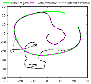
Figure 3 Tracking of a path #1 trajectory in presence of wheels’ slip with and without using slip estimator.

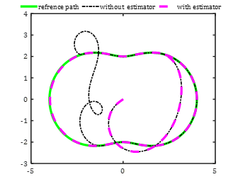
Figure 4 Tracking of a path #3 trajectory in presence of wheels’ slip with and without using slip estimator.

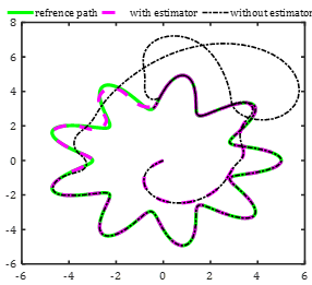
Figure 5 Tracking of a path #2 trajectory in presence of wheels’ slip with and without using slip estimator.

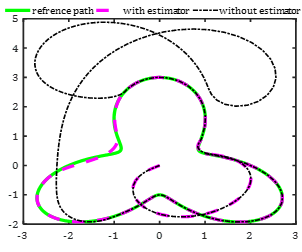
Figure 6 Tracking of a path #4 trajectory in presence of wheels’ slip with and without using slip estimator.

As shown in ‎0, as long as it is in the kinematic design for a situation where adaptive rules prevent the robot from deviating from the reference path if this sensor is deactivated and the uncertainty is applied to the system. The system is capable of to compensate for these disturbances, it is not included in the distance, but in cases where the slip is still not logged in, the robot will continue to follow its path easily and without any problems. Here, the concept and function of the design of an adaptive controller are needed, and to the intensity of the system, especially in large disturbances, depends on this function for the correct behavior and stability of the path. Time-history of system position and orientation errors is shown in ‎0 and ‎0 respectively.

In Figure 7, the robot position signal errors in pursuit of the path in the state of disturbance as a slip and without the estimator and the presence of the uncertainty estimator. And in Figure 8, the robot angle error signals are tracked in a disturbance mode as an uncertainty and without an estimator, as well as the presence of an uncertainty estimator. The control inputs are also designed in Figure 9 by uncertainty in two states with the slip estimator activated and the other without the estimator. This in both cases shows the convergence of the system even by uncertainty. As can be seen, the error signals strating from initial nonzero values converge to the zero after about 20 seconds. Also the control signals have appropriate values and have smooth profiles. The stability and convergance of the signals are also evident from the obtained results. Figure 10 also shows the slip estimator to eliminate the slip of the wheels applied to the system kinematics.

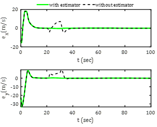
Figure 7 Time-history of system position errors.

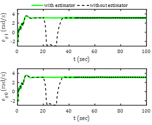
Figure 8 Time-history of system orientation errors.

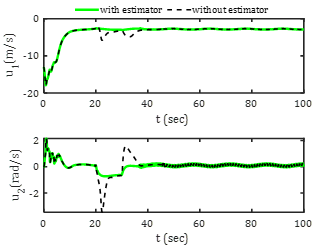
Figure 9 System kinematic control inputs.

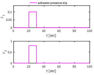
Figure 10 Slip estimator.

In this paper, first, the kinematic model of a wheeled mobile robot with differential thrust is described. Then a dynamic feedback linearization controller is provided that universally ensures the stability of all mode variables. The purpose of this study was to investigate the tracking control of a tractor-trailer wheeled mobile robot using the linearization method of dynamic feedback in the presence of uncertainties in linear input speed and rotational speed. The tractor trailer system is a two-wheeled differential robot with a trailer. This is a highly pragmatic system that is highly nonlinear and subject to non-holonomic constraints. The first system modeling was performed. Then, a dynamic feedback linearization algorithm was introduced to control the tractor-trailer robot tracking. Then, to estimate the uncertainties, a kinematic estimation method was performed to compensate for these effects used to analyze the stability of the closed-loop system. Finally, show results were presented and discussed. The results shown well show the efficiency of the proposed control algorithm and adaptive controller for uncertainty estimation.

None.

The author(s) declared no potential conflicts of interest with respect to the research, authorship, and/or publication of this article.

1. Sun S. Designing approach on trajectory-tracking control of mobile robot. Robotics and Computer-Integrated Manufacturing. 2005;21(1):81‒85.
2. Russo S. Design of a robotic module for autonomous exploration and multimode locomotion. IEEE/ASME Transactions on Mechatronics. 2012;18(6):1757‒1766.
3. Alipour K, Robat A B, Tarvirdizadeh B et al. Dynamics modeling and sliding mode control of tractor-trailer wheeled mobile robots subject to wheels uncertainty. Mechanism and Machine Theory. 2019;138:16‒37.
4. Binh N T, Tung N A, Nam D P, et al. An adaptive backstepping trajectory tracking control of a tractor trailer wheeled mobile robot. International Journal of Control, Automation and Systems. 2019;17(2):465‒473.
5. Wang C, Liu X, Yang X, et al. Trajectory tracking of an omni-directional wheeled mobile robot using a model predictive control strategy. Applied Sciences. 2018;8(2):231.
6. Xie Y. Coupled fractional-order sliding mode control and obstacle avoidance of a four-wheeled steerable mobile robot. ISA transactions. 2021;108:282‒294.
7. Madanzadeh S, Abedini A, Radan A, et al. Application of quadratic linearization state feedback control with hysteresis reference reformer to improve the dynamic response of interior permanent magnet synchronous motors. ISA transactions. 2020;99:167‒190.
8. Hmidi R, Brahim AB, Hmida FB, et al. Robust fault tolerant control design for nonlinear systems not satisfying matching and minimum phase conditions. International Journal of Control, Automation and Systems. 2020;18(9):2206‒2219.
9. Gandomi AH, Alavi AH. A new multi-gene genetic programming approach to nonlinear system modeling. Part I: materials and structural engineering problems. Neural Computing and Applications. 2012;21(1):171‒187.
10. Preece R, Huang K, Milanović J V et al. Probabilistic small-disturbance stability assessment of uncertain power systems using efficient estimation methods: IEEE Transactions on Power systems. 2014;29(5):2509‒2517.
11. de Jesús Rubio J. Robust feedback linearization for nonlinear processes control. ISA transactions. 2018;74:155‒164.
12. Onorio M D, Caruso G. Safety Analyses with uncertainty quantification for fusion and fission nuclear power plants. Applications to EU DEMO fusion reactor and BWRs; 2020. 1‒176 p.
13. Lurie B, Enright P. Classical Feedback Control: With MATLAB® and Simulink®. CRC Press, 2011.
14. Yuan X, Chen Z, Yuan Y, et al. Sliding mode controller of hydraulic generator regulating system based on the input/output feedback linearization method. Mathematics and Computers in Simulation. 2016;119:18‒34.
15. Li S E, Qin X, Li K, et al. Robustness analysis and controller synthesis of homogeneous vehicular platoons with bounded parameter uncertainty. IEEE/ASME Transactions on Mechatronics. 2017;22(2):1014‒1025.
16. Yu W, Jafari R. Modeling and Control of Uncertain Nonlinear Systems with Fuzzy Equations and Z-Number. John Wiley& Sons; 2019. 208 p.
17. Mo H, Farid G. Nonlinear and adaptive intelligent control techniques for quadrotor uav–a survey. Asian Journal of Control. 2019;21(2):989‒1008.
18. Neher M, Jackson K R, Nedialkov N S. On Taylor model based integration of ODEs. SIAM Journal on Numerical Analysis. 2007;45(1):236‒262.
19. Lee T C, Song K T, Lee C H, et al. Tracking control of unicycle-modeled mobile robots using a saturation feedback controller. IEEE transactions on control systems technology. 2001;9(2):305‒318.
20. Sarkar N, Yun X,  Kumar V. Control of mechanical systems with rolling constraints. Application to dynamic control of mobile robots: The International Journal of Robotics Research. 1994;13(1):55‒69.
21. Khalaji A K, Jalalnezhad M. Stabilization of a Tractor with n Trailers in the Presence of Wheel Uncertainty Effects. Robotica. 2020;39(5):1‒11.