The concept of an intelligent control system for a complex nonlinear biomechanical control object of an extension cableless robotic unicycle is considered. A thermodynamic approach to study optimal control processes in complex nonlinear dynamic systems is applied. The results of stochastic simulation of a fuzzy intelligent control system for various types of external/internal excitations for a dynamic, globally unstable control object-extension cableless robotic unicycle based on Soft Computing (Computational Intelligence Toolkit) technology are presented¹. A new approach to design an intelligent control system based on the principle of the minimum entropy production (minimum of useful resource consumptions) determination in the control object movement and the control system is developed. This determination as a fitness function in the genetic algorithm to achieve robust control of a robotic unicycle is used. An algorithm for entropy production calculation and representation of their interrelationship with the Lyapunov function (a measure of stochastic robust stability) is described.

Keywords: robotics unicycle, intelligent control systems, essentially nonlinear model, globally unstable model, stochastic simulation, soft computing

¹Some results received during the Ph.D. course in University of Electro-Communications, Dept. of Mechanical and Intelligent Control Eng., Tokyo, Chofu, Japan, the supervisor prof. K. Yamafuji.

Intelligent mechatronics as background of new types of nonlinear mechanical systems motion - modern methods and algorithms of intelligent control’s development.

The extraction of knowledge from a new movement types is based on studding of mathematical model benchmarks. The robotic unicycle motion is one of such type of “benchmark movements” (benchmark model of nonlinear mechanics),^1–5 described as nonlinear nonholonomic, global unstable dynamic system. Related research of such dynamic systems is interesting for nonlinear mechanics (to develop a new method of nonlinear effects research) and for modern control theory (to deve1op a new intelligent control algorithms).

Development of an algorithm and control system for robotic unicycle benchmark required а new computation technology-computational intelligence. The physical feature of robotic-unicycle is that the real unicycle bike’s control is realized by skillful human operator only. This leads to the studding of the robotic unicycle as a biomechanical system including new approaches to the control system, such as intuition, instinct and emotions inherent to the human-operator (rider) and allowing to study the possibility of cognitive control by including the “human factor” in the control circuit. The control of the robotic unicycle motion is based on the coordination of the complex movement components (pedaling and movement of the rider’s torso). Changing the components coordination type generates new types of movement (rectilinear movement, slalom, dance, jumping, etc.).

Related works

Previous studies conducted in the field of different unicycle robot’s models controlling (Figure 1) considered the system only from the viewpoint of a mechanical model using classical control methods and/or a simplified, mixed fuzzy proportional-differential controller (FPD) with empirical tables of fuzzy decision rules (lookup tables).^1–4 However, this becomes an algorithmically insoluble problem for traditional control methods in the task of robust (stable) motion of the object and has resulted in new approaches appearance to solve this issue.

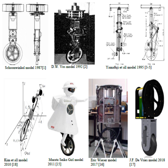
Figure 1 Another model of unicycle robot for previous years.

The conceptual structure of robotic unicycle intelligent control system research and development is shown in Figure 1A.

To solve this controlling problem the cyber-physical model called as “Conceptual Logical Structure of the Distributed Knowledge Representation (Information Levels) in the Artificial Life of the Robotic Unicycle” (Figure 1A&1B) as a biomechanical model of object movement and control was developed and proposed.

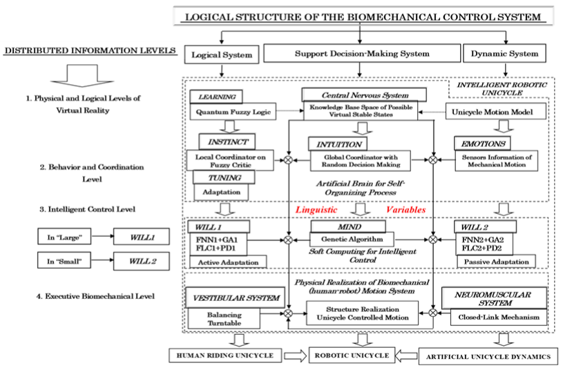
Figure 1A Conceptual Logical Structure of Distributed Knowledge Representation (on Information Levels) in Artificial Life of the Robotic Unicycle.

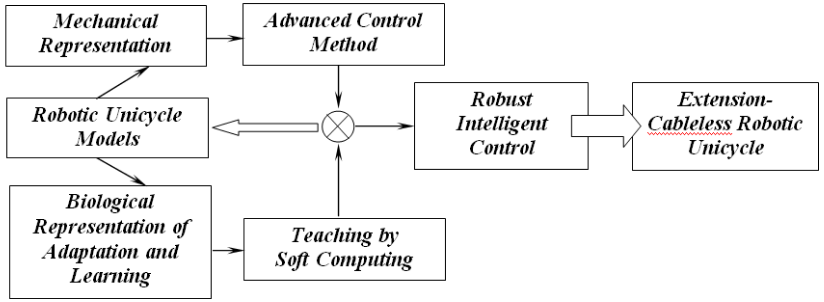
Figure 1B The conceptual scheme of the Robotic Unicycle R&D.

Studying the control problem of the robotic unicycle nonlinear biomechanical model, as well as the creation and "training" of a control system by means of available soft computing methods and algorithms was a main research goal.

To assess the control quality the new physical principle the minimum entropy production rate in the object’s movement and in the control system^2–13 is introduced. The physical measure of entropy production rate is applied as a fitness function in the genetic algorithm (GA). This approach ensures the global stability of the dynamic control object and control system’s robustness. Basing on this approach the “Self-organizing structure of an artificial intelligent (AI), robust control system design with a new physical measure of control quality” (Figure 2) with a new type of intelligent feedback rooted in the principles of computational intelligent, as well as “Fuzzy Simulation structure of an intelligent control system design with soft computing algorithms (Figure 3) has been developed.

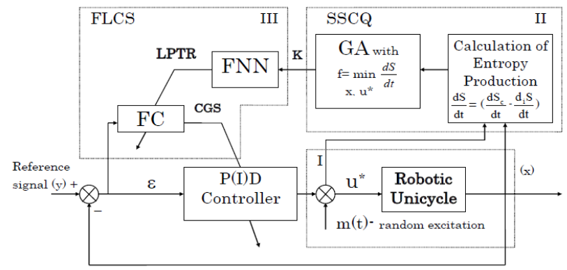
Figure 2 “Self-organizing structure of an artificial intelligent (AI), robust control system design with a new physical measure of control quality”.
Description: GA, Genetic Algorithm; f, Fitness Function of GA; S, Entropy of System; Sc, Entropy of Controller; Si, Entropy of Controlled Plant; ε, Error; u, Optimal Control Signal; m(t), Disturbance; FC, Fuzzy Controller; FNN, Fuzzy Neural Network; FLCS, Fuzzy Logic Classifier System; SSCQ, Simulation System of Control Quality; K, Global Optimum Solution of Coefficient Gain Schedule (Teaching Signal); LPTR, Look-up Table of Fuzzy Rules; CGS; Coefficient Gain Schedule K=(k1,k2,k3,k4).

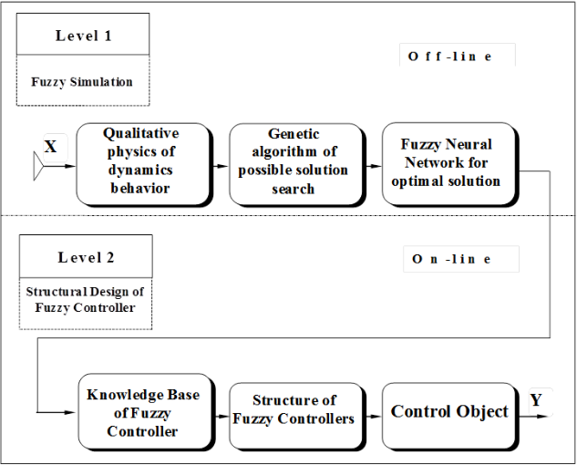
Figure 3 Fuzzy Simulation structure of an intelligent control system design.

In previous studies, the problem of external and internal excitations in the mechanical and control system was not considered, see.^1–4 As a result, the global dynamic stability in object’s control was not achieved.

In this article the modeling and optimization of intelligent control system with simulation of stochastic external\internal excitations in the mechanical and control systems (floor roughness’s, mechanical vibrations, zero sensors drift etc.) using the structure of the forming filters⁵ is represented.

The simulation and experiment results confirming the efficiency of the robotic unicycle control system.

As it’s mentioned above, the objective of this research is development the intelligent control system for non-holonomic, essentially nonlinear, global spatially unstable, highly linking constrained model of the robotic unicycle. For this purpose, a new unicycle mathematical model was created for the “Real” unicycle’s coordinate system Figure 4.

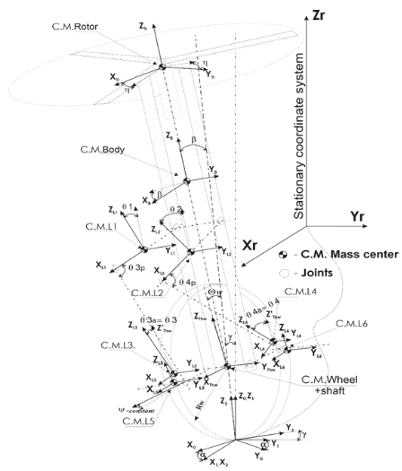
Figure 4 Coordinates description of the robotic unicycle model.

For this coordinate system the following explanations for basic and generalized coordinates, generalized velocities and accelerations is derived:

Elemental Coordinates-$q_j(t)=[x0,y0,\alpha ,\gamma ,\beta ,\theta w,\Psi ,\theta 1,\theta 2,\theta 3,\theta 4,\eta ]$ ;where j=1,…,12

$\Psi (t)=\theta w(t)+\psi (const)$ ,$\frac{dx0(t)}{dt}=Rw\cdot \frac{d\theta w(t)}{dt}\cdot \cos (\alpha (t))$ ; $\frac{dy0(t)}{dt}=Rw\cdot \frac{d\theta w(t)}{dt}\cdot \sin (\alpha (t))$ $\psi (const)$ - initial position of pedals Figure 4 (link 5,6).Hereinafter, the indices (i, j) denotes the serial numbers of elements in the corresponding vectors, matrices, and in the system equations

The equation of non-holonomic constraints in case of unslipping rolling between wheel and ground:

$\frac{dx0(t)}{dt}=Rw\cdot \frac{d\theta w(t)}{dt}\cdot \cos (\alpha (t))$ ;$\frac{dy0(t)}{dt}=Rw\cdot \frac{d\theta w(t)}{dt}\cdot \sin (\alpha (t))$ (1.1)

where Rw – wheel radius, $\dot{\theta }w(t)$ - velocity of wheel rotation,$\alpha (t)$ - yaw angle. The coordinates x0, y0 are eliminated by substituting of Eq. (1.1) to kinematic Lagrangean part.

Generalized Coordinates$q_j(t)=[\alpha ,\gamma ,\beta ,\theta w,\theta 1,\theta 2,\theta 3,\theta 4,\eta ]$ , j = 1,…,9.

In Figure 4 notation:$a$ - yaw angle;$\gamma$ - roll angle; $\beta$ - pitch angle; C.M. – center of mass; L 1,…,6 – links 1-6;  ${\theta }_w$ wheel rotation angles; $\theta$ 1, …,4 – links rotation angles; $\Psi$ - initial position of pedals andthe current angle of pedal rotation (link 5,6) is included in equations as summa - $\Psi (t)=\theta w(t)+\psi (const)$ .

Thus, the Lagrangian solvation with insertion represented above equations of nonholonomic/holonomic constraints and external forces of stochastic excitations, gives the following generalized stochastic equation of the robotic unicycle system motion with control:

$\{\begin{array}{l}M{E}_{i,j}(q)\cdot {\ddot{q}}_j^T(t)={\tau }^T{}_i+C^T{}_i(q,\lambda )+{\xi }^T{}_i(t)-(B{T}_{i,j}(q,\dot{q})\cdot {\dot{q}}_j^T(t)+G^T{}_i(q)+D^T{}_i(\dot{q}))\text{ (a)}\\ A_{i,n}(q)\cdot {\lambda }_n=M{c}_{i,j}(q)\cdot {\ddot{q}}_j^T(t)+B{c}_{i,j}(q,\dot{q})\cdot {\dot{q}}_j^T(t)+G{c}^T{}_i(q)+D{c}^T{}_i(\dot{q})-\tau c^T{}_i-\xi c^T{}_i(t)\text{ (b)}\end{array}$ (1.2)

where - i,j=1..9; vector of generalized accelerations ${\ddot{q}}_j(t)=[\ddot{\alpha },\ddot{\gamma },\ddot{\beta },\ddot{\theta }w,\ddot{\theta }1,\ddot{\theta }2,\ddot{\theta }3,\ddot{\theta }4,\ddot{\eta }]$ ; vector of generalized velocities ${\dot{q}}_j(t)=[\dot{\alpha },\dot{\gamma },\dot{\beta },\dot{\theta }w,\dot{\theta }1,\dot{\theta }2,\dot{\theta }3,\dot{\theta }4,\dot{\eta }]$ . In the system of equations Eq (1.2), equation (a) is the dynamical equation of motion for the whole unicycle model with stochastic excitations, and equation (b) is the description of Lagrangian multipliers ${\lambda }_n$ , where n=1…4. Matrices, vectors and another terms of equations (1.2) described in detail in the following sections of this article.

Stochastic excitation appears in case of $\xi c_i(t)$ &${\xi }_i(t)$ ≠ 0 and described via differential equation of Forming Filter as Gaussian (as in our case) random process with autocorrelation function $R({{\tau }^{\prime }}_{\xi }^{})={\sigma }_{\xi }^2\cdot \exp (-{\alpha }_{\xi }\cdot \left|{{\tau }^{\prime }}_{\xi }^{}\right|)$ . This disturbance is included into equation of motion for some generalized coordinates, and it is modelling the possible roughness of flow, jamming in closed-links mechanism, and inaccuracy of angular acceleration measuring (sensors zero drift).

Under these conditions’ the stochastic equation of motion with parametric excitations is obtained. All of this gives a possibility to simulate behavior of dynamic controlled system more realistically and determine the real parameters of intelligent controllers for error estimation and control robustness. Stochastic modelling via Forming Filters is described below in.⁵

For (un)stability definition the Salvadory theorem about equilibrium of mechanical systems with dissipative forces of a $Q_i(q,\dot{q})$ type along with full energy of system $E(q,\dot{q})$ as Lyapunov function$V(q,\dot{q})\equiv E(q,\dot{q})=T(q,\dot{q})+U(q)$ is used; where $T(q,\dot{q})$ is system kinetic energy, $U(q)$ - potential energy of system. Under Lyapunov’s theorem conditions, if the function $V(q,\dot{q})$ is:

positively determined about any q,$\dot{q}$ and have 0 at $(q,\dot{q})=0$ , i.e. $V(q,\dot{q})\ge a\Vert (q,\dot{q})\Vert$ &$V(0)=0$ , where a is a some continuous, strictly increasing function, satisfying to a condition $a(0)=0$ ;

Derivative of function V by time t is negative, i.e. $\dot{V}(q,\dot{q})\le 0$ ; when origin is stable:⁶

Let’s considering conditions of Salvadori's theorem that determine the dynamical systems stability, Assume if:

U(q) have minimum at $q=0$ ;

U(q) don’t have minimum at $q=0$ ;

equilibrium statement $q=0$ is insulated;

Absolute dissipation $(Q|\dot{q})\le -a\Vert \dot{q}\Vert$ , where a is a strictly positive definite function.

Then with conditions

Equilibrium state $(q,\dot{q})=0$ is stable; in the case, with condition equilibrium state $(q,\dot{q})=0$ unstable.

Basing on the both theorems lets define a stability condition of the robotic unicycle system. The equation for expression of robotic unicycle potential energy for $q_j=(0,0,0,0,\theta 1,\theta 2,\theta 3,\theta 4,0)$ has following form:

${\displaystyle \sum _n{U}_n(0)=g\cdot [Rw\cdot {\displaystyle \sum _n{{\rm M}}_n}+{{\rm M}}_3\cdot (2\cdot e1-e2\cdot (\sin (\theta 1)+\sin (\theta 2)))+\Delta z\cdot {{\rm M}}_5\cdot (\cos (\theta 3)+\cos (\theta 4))+{{\rm M}}_7\cdot e6]}$     (2.1)

where: coordinates $\theta 1,\theta 2,\theta 3,\theta 4$ - cannot be equal to 0 at $\gamma ,\beta ,\theta w=0$ by mechanical constraints of closed-links mechanism; $M_i$ - masses of robotic unicycle parts; $Rw,e1,e2,e6, \Delta z$ - sizes in Figure 4. From Eq. (2.1) follows, that $U\left(0\right)$ has maximumvalue in the equilibrium statement. The Eq. (2.1) satisfies to condition 1a) of Salvadory theorem, that describes instability of robotic unicycle system at equilibrium statement. This enables to assert about global instability of the robotic unicycle dynamic system. However, as discussed in,⁶ in case if the $U\left(0\right)$ has maximum value it possible that the equilibrium will stable owing to occurrence of external forces, such as gyroscopic or similar that in our case is controlled torques.

This research proclaims that it is possible to create such intelligent control system, which can continuously stabilize dynamic motion of nonlinear robotic unicycle and the simulation results approved these are shown below.

To provide computational intelligence methods that can coordinating the complex motion components, it is necessary to use qualitatively new control algorithms that can operate with linguistic variables.⁸ Soft computing methods fully satisfy to these requirements and that are determines their use. Basing on the physical and sophisticated description of the biomechanical model, and using soft computing methods, the following structure of modeling the intelligent control system is represented.

Biomechanical model of intelligent control system

The human riding control of the unicycle as logic-dynamic hierarchical process may be formed by:

1. mechanical dynamic system "human-rider-unicycle";
2. decision-making process of unicycle intelligent control with different levels of “riding skills”;
3. logical behavior for human body motorists (legs, hands and torso coordination) based on intuition, instinct, and emotion mechanisms;
4. distributed information system for cooperative coordinating of sub-systems in biomechanical model.⁸

In accordance with this representation of dynamic control process a hierarchical logic structure of distributed knowledge representation of the robotic unicycle artificial life is shown in Figure 1. For description of artificial life of robotic unicycle, the methods of qualitative physics for internal world representation based on mathematical model of unicycle motion used.

Logic structure of biomechanical control system for description a human riding of unicycle includes four levels:

1. distributed information levels with sub-levels;
2. logical system;
3. support decision-making system;
4. dynamic mechanical system.

Further the proposals of this structure are described in details. Distributed information levels include four sub-levels:

1. physical level and logic of virtual reality;
2. behavior and coordination level;
3. intelligent control levels with two sub-levels;
4. executive biomechanical level.

Intersections between the horizontal lines of distributed information levels and vertical lines of logical system, support decision-making system, and dynamic system (of unicycle motion and a human-rider behavior as biomechanical control model) realize the particular for human unicycle riding models with different skill levels of smart control tools using. Let’s consider here this approach with examples.

Example 1: Physical and logical level of virtual reality. The intersection of the first horizontal level (Physical and logical level of virtual reality) with the first vertical level (Logical system) gives the structure of the human learning process to ride (control) a unicycle. The intersection with the second vertical level (support decision making system) corresponds to the level of the central nervous system (CNS) as a biological control system. The intersection with the third level (Dynamic (mechanical) system) is introduced mechanical model of the of a unicycle movement as a dynamic system. The logical sum of these sublevels implements the physical level of the unicycle movement description and the physical interpretation of the experimental data (attempts). The mathematical background for describing the learning process is the quantum fuzzy logic. The functions of the CNS are realized as the knowledge base (KB) domain of possible stable states. But, to create a control system of such a high intelligent level is not currently possible.

Example 2: Behavior and coordination level. This structure includes the mechanisms of instinct, intuition and emotion. The mechanism of instinct is described in the logical structure as a local coordinator with fuzzy rules and corresponds to a control structure with active and passive adaptation based on a fuzzy neural network (FNN). The mechanism of intuition is represented as a global coordinator and realized in the control process as a decision-making process based on a genetic algorithm (GA). The mechanism of emotions is described basing on the information from motion sensors and represented in the form of lookup tables with different semantic expression of the linguistic description of the desired dynamic motion behavior (as examples, "smoothly", "quickly" and so on). Thus, the intersection of two distributed information levels with logical systems is realizing the artificial brain unit for the process of unicycle control system self-organization.

Example 3: The Intelligent control level - an artificial intelligent control system with a distributed knowledge representation, includes “will” and “mind” (desires and opportunities) concepts, just like a human being.^9,10 For the mechanisms of instinct and emotion, new lookup tables are determined using an FNN. The mechanism of intuition is realized on the GA basis and directs the two fuzzy controllers’ actions. Thus, the fuzzy simulation based on mathematical GA and FNN tools implements the soft computing algorithm in the robot’s intelligent control system.

From a qualitative physical description and movement simulation the domain of possible virtual stable states described by a strange attractor is obtained, as it was shown in.^3,4 This suggests that the human postural control system is highly organized complex system and the position of the human body changes (sways) stochastically. This fully corresponding to the results described in.¹¹

Example 4: Executive biomechanical level - the physical process of the robotic unicycle system realization. In this case, the vestibular system as a logical control structure is realized by the balancing turntable (torso, shoulder girdle and arms), and the neuro-muscular system is formed by the closed-links mechanism of the legs.

Thus, the dynamic process of human unicycle riding control with different intelligent behavior levels should be described as the intersection of logical systems with distributed information levels.

The intelligent robust control system structuring

The development of robust control for complex dynamic systems motion has two ways of research:

1. The study of stable motion processes,
2. The study of unstable motion processes of complex dynamic systems.

As mentioned above, our attention has been focused on the study of the robotic unicycle as a dynamic, global-spatially unstable controlled object. Such a global-spatially unstable dynamic object requires a new intelligent robust control algorithm based on knowledge description of an essentially nonlinear, unstable dynamic system movements.^3,8 The structure of the intelligent robust control algorithm in the conceptual form for the entire class of unstable dynamic control objects was described in^{2–4, 8} and here we apply it to the problem of controlling the robotic unicycle.

The control structure with a new intelligent feedback type is represented in Figure 2. It is based on the scheme of a conventional control system with linear feedback P(I)D, intelligent soft computing tools (fuzzy set theory, fuzzy neural networks (FNN), genetic algorithms (GA)); nonlinear model of the control object; entropy production rate calculating; stochastic simulation of random external/internal excitations.

In the structure Figure 2 the following designations are used: GA - Genetic Algorithm; f - Fitness Function of GA;S- Entropy of System; $S_c$ - Entropy of Controller; $S_i$ - Entropy of Controlled Plant; $\epsilon$ - Error; u*- Optimal Control Signal; m(t) – Disturbances (random external/internal excitations); FC - Fuzzy Controller; FNN - Fuzzy Neural Network; FLCS - Fuzzy Logic Classifier System; SSCQ - Simulation System of Control Quality; K - Global Optimum Solution of Coefficient Gain Schedule (Teaching Signal); LPTR - Look-up Table of Fuzzy Rules; CGS - Coefficient Gain Schedule (in case of 2 PD controllers -$K=\left(k_1,k_2,k_3,k_4\right))$ .

The self-organization control in this system, at the first stage, is provided by optimizing the control parameters of the P(I)D controller by selecting the best solutions with a genetic algorithm, in which the selection criterion is the best fitted solution, calculated using the fines function. To determine solution fitness’s a new physical measure of control quality is used -the entropy production minimum rate. This measure is a difference between entropy production of the control object itself and the control system included in this object. This allows adapting the parameters of the linear control system to a nonlinear control object.^7,12

The next adaptation stage is control system training to ensure its robustness. This step is based on a fuzzy logic classifier that defines fuzzy rules for logical relationships of linear controller parameters. The classifier in this step is FNN for which the optimized control parameters obtained from the genetic algorithm output are used as the training signals. This stage generates fuzzy lookup tables, adapted control parameters of the low-level controller P(I)D.

In this approach, for the task of nonlinear object controlling, the criterion of the control quality (controllability) is introduced as the entropy production function, which is directly interrelated with the Lyapunov function i.e. to a dynamic system stability, as it shown in.^7,12,13 The interrelation between these functions in an intelligent control system ensures its robustness, as shown in Figure 5. Further, the obtained lookup tables are used by a fuzzy controller (FC) to control the linear controller parameters (PD).

Figure 5 Interrelation structure between a Stability, Robustness and Controllability of the system.

Based on the intelligent control structure and interrelationship in Figure 5, the Fuzzy Simulation structure of an intelligent control system design was developed in Figure 3.

Simulation is decomposed into follow main stages: Off-Line and On-Line. At the first stage a controlled object as the mathematical model is created and the thermodynamic equations of its states are founded for entropy calculation. Further, the equations for entropy production are forming the GA’s fitness function. The GA in computer stochastic simulation mode optimizing the P(I)D controller’s parameters. The next step is the training of the control system based on the optimized controller parameters obtained from the GA and obtaining lookup tables (FC Knowledge Base) using the FNN.

In On-Line mode, the P(I)D controller’s parameters of the robotic unicycle are changes by a fuzzy controller basing on the obtained lookup tables, in real time. The structure of the robot control system is described below.

The simulation basis is the mathematical model described the control object motion and represented in (1.2). Let us dwell on the equations (1.2) description.

For the mathematical simulation of a robotic unicycle movement the following parameters of the model (1.2) are adopted and graphically represented in Figure 4: where - i,j= 1 ... 9; ${\ddot{q}}_j(t)=[\ddot{\alpha },\ddot{\gamma },\ddot{\beta },\ddot{\theta }w,\ddot{\theta }1,\ddot{\theta }2,\ddot{\theta }3,\ddot{\theta }4,\ddot{\eta }]$ - vector of generalized accelerations; ${\dot{q}}_j(t)=[\dot{\alpha },\dot{\gamma },\dot{\beta },\dot{\theta }w,\dot{\theta }1,\dot{\theta }2,\dot{\theta }3,\dot{\theta }4,\dot{\eta }]$ - vector of generalized velocities; In the system of equations Eq(1.2), equation (a) is the dynamic equation of motion for the whole unicycle model, and equation (b) is the description of Lagrangian multipliers ${\lambda }_n$ , where n=1... 4.

In Eq.(1.2,a), $M{E}_{i,j}\left(q\right)$ is a 9X9 block matrix that consists of inertial acceleration’s terms $M\left(q\right)$ , derived from Lagrange equations, and geometricalacceleration’s terms derived from equations of closed-links mechanism constraints $E\left(q\right)$ ; $B{T}_{i,j}(q,\dot{q})$ is a 9X9 blockmatrix that consists of Coriolis and centrifugal $B(q,\dot{q})$ &$T(q,\dot{q})$ terms, derived from Lagrange equations, and equations of closed-links mechanism constraints, respectively; $G_i\left(q\right)$ is a 9-dimensional vector of gravity terms $G_i(q)=[0,G_2(q),G_3(q),G_4(q),0,0,0,0,0]$ ;$D_i(q,\dot{q})$ is a 9-dimensional vector of viscous friction forces terms $D_i(\dot{q})=[D_1(\dot{q}),D_2(\dot{q}),D_3(\dot{q}),D_4(\dot{q}),0,0,0,0,D_9(\dot{q})]$ ;${\tau }_i$ is a 9-dimensional vector of torque ${\tau }_i=[0,0,0,0,0,0,0,0,{\tau }_{(\eta )3}]$ ; $C_i(q,\lambda )$ is 9-dimensional vector of Lagrangian multipliers with respected coefficients of constraint equations $C_i(q,\lambda )=[0,0,C_{(\beta )1},C_{(\theta w)2},0,0,0,0,0]$ ; ${\xi }_i(t)$ is 9-dimensional vector of given stochastic excitation.

$M{E}_{i,j}(q)=\left[\begin{array}{cccccc}{M}_{11}(q)& \mathrm{..}& \mathrm{..}& \mathrm{..}& \mathrm{..}& M_{19}(q)\\ \mathrm{..}& \mathrm{..}& \mathrm{..}& \mathrm{..}& \mathrm{..}& \mathrm{..}\\ M_{41}(q)& \mathrm{..}& \mathrm{..}& \mathrm{..}& \mathrm{..}& M_{49}(q)\\ 0& 0& E_{53}(q)& \mathrm{..}& E_{58}(q)& 0\\ \mathrm{..}& \mathrm{..}& \mathrm{..}& \mathrm{..}& \mathrm{..}& 0\\ 0& 0& E_{83}(q)& \mathrm{..}& E_{83}(q)& 0\\ M_{91}(q)& \mathrm{..}& \mathrm{..}& \mathrm{..}& \mathrm{..}& M_{99}(q)\end{array}\right]\text{ ;}$

$B{T}_{i,j}(q,\dot{q})=\left[\begin{array}{cccccc}{B}_{11}(q,\dot{q})& \mathrm{..}& \mathrm{..}& \mathrm{..}& \mathrm{..}& B_{19}(q,\dot{q})\\ \mathrm{..}& \mathrm{..}& \mathrm{..}& \mathrm{..}& \mathrm{..}& \mathrm{..}\\ B_{41}(q,\dot{q})& \mathrm{..}& \mathrm{..}& \mathrm{..}& \mathrm{..}& B_{49}(q,\dot{q})\\ 0& 0& T_{53}(q,\dot{q})& \mathrm{..}& T_{58}(q,\dot{q})& 0\\ \mathrm{..}& \mathrm{..}& \mathrm{..}& \mathrm{..}& \mathrm{..}& 0\\ 0& 0& T_{83}(q,\dot{q})& \mathrm{..}& T_{83}(q,\dot{q})& 0\\ B_{91}(q,\dot{q})& \mathrm{..}& \mathrm{..}& \mathrm{..}& \mathrm{..}& B_{99}(q,\dot{q})\end{array}\right]\text{ ;}$

In Eq.(2,b), $M{c}_{i,j}\left(q\right)$ is a 9X9 matrix of inertial acceleration’s terms $M\left(q\right)$ derived from Lagrange equations; $B{c}_{i,j}(q,\dot{q})$ is a 9X9 matrix of Coriolis and centrifugal $B(q,\dot{q})$ terms, derived from Lagrange equations;$G{c}_i\left(q\right)$ is a 9-dimensional vector $G{c}_i(q)=[0,0,0,0,G_5(q),G_6(q),G_7(q),G_8(q),0]$ of gravity terms; $D{c}_i(q,\dot{q})$ is a 9-dimensional vector $D{c}_i(\dot{q})=[0,0,0,0,D_5(\dot{q}),D_6(\dot{q}),D_7(\dot{q}),D_8(\dot{q}),0]$ of viscous friction forces terms; $\tau c_i$ is a 9-dimensional vector of torque $\tau c_i=[0,0,0,0,0,0,{\tau }_{(\theta 3)1},{\tau }_{(\theta 4)2},0]$ ; $\xi c_i(t)$ is given stochastic excitation; $A_{i,n}\left(q\right)$ is a 9X4 matrix of geometricalterms derived from constraints equations of closed-links mechanism, correspond to motion equation by i index; ${\lambda }_n$ - 4-dimensional vector of Lagrangian multipliers:

$M{c}_{i,j}(q)=\left[\begin{array}{ccc}0& \mathrm{..}& 0\\ \mathrm{..}& \mathrm{..}& \mathrm{..}\\ M_{51}(q)& \mathrm{..}& M_{59}(q)\\ \mathrm{..}& \mathrm{..}& \mathrm{..}\\ M_{81}(q)& \mathrm{..}& M_{89}(q)\\ 0& \mathrm{..}& 0\end{array}\right]\text{ ;}$ $B{c}_{i,j}(q,\dot{q})=\left[\begin{array}{ccc}0& \mathrm{..}& 0\\ \mathrm{..}& \mathrm{..}& \mathrm{..}\\ B_{51}(q,\dot{q})& \mathrm{..}& B_{59}(q,\dot{q})\\ \mathrm{..}& \mathrm{..}& \mathrm{..}\\ B_{81}(q,\dot{q})& \mathrm{..}& B_{89}(q,\dot{q})\\ 0& \mathrm{..}& 0\end{array}\right]\text{ ;}$

$A_{i,n}(q)=\left[\begin{array}{cccc}0& 0& 0& 0\\ \mathrm{..}& \mathrm{..}& \mathrm{..}& \mathrm{..}\\ A_{51}(q)& A_{52}(q)& 0& 0\\ 0& 0& A_{63}(q)& A_{64}(q)\\ A_{71}(q)& A_{72}(q)& 0& 0\\ 0& 0& A_{83}(q)& A_{84}(q)\\ 0& 0& 0& 0\end{array}\right]$

The equations of the Robotic Unicycle system’s controlled torques

In the case of PD controller for the Links mechanism, the controlled torque is given as:

${\tau }_{(\theta 3)1}={\tau }_{(\theta 4)2}=-kp1(T)\cdot \beta (t)-kd1(T)\cdot \dot{\beta }(t)$ (4.1)

and for the Rotor mechanism - as:

${\tau }_{(\eta )3}=kp2(T)\cdot \gamma (t)+kd2(T)\cdot \dot{\gamma }(t)$ (4.2)

GA generates P(I)D controller's parameters $kp1(T),kp2(T),kd1(T),kd2(T)$ , selecting them basing on the results of the fitness function calculations, each sampling time T=0.05sec. This sampling time is defined from real controller scheme of Robotic Unicycle.

Information-thermodynamic criterion of the control qualities distribution

The thermodynamic ratio between the robust intelligent control quality and the optimization criterion, used in the quantum algorithm (QA) of a self-organization knowledge bases (KB),¹ are shown in Table 1.

Table 1 Thermodynamic ratio of a robust intelligent control quality distribution

In Table 1 the following notations are introduced: $V$ - Lyapunov function; $S_{ОУ},S_{Р}$ entropy production in the Control Object & Controller, respectively; $V=\frac{1}{2}{\displaystyle \sum _{i=1}^n{q}_i^2}+\frac{1}{2}{S}^2;S=S_{ОУ}-S_{Р};{\dot{q}}_i=\phi \left(q_i,u,t\right)$ -the control object’s equation of motion; $q_i$ - generalized coordinates; $u$ - the desired control.

In the Table 1 the equation of dynamic system control qualities distribution connecting, in an analytical form, such a qualitative notions of control theory as - stability, controllability and robustness, basing on the phenomenological thermodynamics entropy concept. As a result, the necessary distribution between the stability, controllability and robustness levels allows achieving the control goals in emergency situations with a minimum of useful resource consumption by using as the GA’s fitness function the criterion of minimum generalized entropy production. The thermodynamic definition of the S and information H entropies are interrelated by the von Neumann relation in the form: $S=kH=-k{\displaystyle \sum _i{p}_i}\ln p_i$ ; where $k\approx 1.38\times {10}^{-23}$ J/K is the Boltzmann constant. As a result (after substitution of this ratio), obtained equation, that also interrelates stability, controllability and robustness but on the basis of the Shannon's information entropy, allows to determine the control to guarantee achievement of the control goal in emergency situations with the requirement of a minimum information quantity about the external environment and Control Object’s states.

Therefore, these ratios are forming an equations system of control definition which are guarantees the control goal achievement in emergency situations with a minimum useful resource consumption and the minimum required initial information.^1–4

Information and thermodynamic distribution of control quality rates

Assume that the control object is described in general form by the equation ${\dot{q}}_i=\phi \left(q,t,S\left(t\right),u\right)$ , where the generalized coordinate $q_i$ describes the control object movement, $u$ is the desired control and $\text{S}\left(t\right)=S_O\left(t\right)-S_C\left(t\right)$ is the generalized entropy of the system represented as the difference between the control object’s entropy production $S_O\left(t\right)$ and the controller’s entropy production $S_C\left(t\right)$ . Consider the following equation:

$\underset{Stability}{\underbrace{\frac{dV}{dt}}}=\underset{\text{Controllability}}{\underbrace{{\displaystyle \sum _{i=1}^n{q}_i\cdot \phi \left(q,t,S\left(t\right),u\right)}}}+\underset{\text{Robustness}}{\underbrace{\left(S_O-S_C\right)\cdot \left({\dot{S}}_O-{\dot{S}}_C\right)}}\le 0$                      (4.3)

Equation (4.3) in analytical form interrelates such qualitative notations of control theory as stability V (Lyapunov function), controllability and robustness basing on the concept of phenomenological thermodynamics entropy.^1–6

This approach allows, as it noted earlier, to find the necessary distribution between the levels of stability, controllability and robustness, which are permits to achieve the control goal in emergency situations with a minimum useful resource consumption by using the minimum generalized entropy production as a fitness function in the genetic algorithm, which is included in the right part Eq. (4.3).

Considering now the (4.3) regarding to the interrelation of thermodynamic entropy S to Shannon information entropy H. The thermodynamic definition of S and H entropies are interrelated by the von Neumann²,³ relation in the:$S=kH=-k{\displaystyle \sum _i{p}_i}\ln p_i$ , where $k\approx 1.38\times {10}^{-23}$ J/K is the Boltzmann constant. Substitution the Shannon information entropy – H instead of $S\left(t\right)$ in equation (4.3) give as a result:

$\underset{\text{Stability}}{\underbrace{\frac{dV}{dt}}}=\underset{\text{Controllability}}{\underbrace{{\displaystyle \sum _{i=1}^n{q}_i\cdot \phi \left(q,t,k\left(H_O-H_C\right),u\right)}}}+k\underset{\text{Robustness}}{\underbrace{\left(H_O-H_C\right)\cdot \left({\dot{H}}_O-{\dot{H}}_C\right)}}\le 0$ (4.4)

Thus, the equation (4.4) also interrelates stability, controllability and robustness, but already on the Shannon’s information entropy basis, which also allows defining controlling approaches for guaranteed achievement of the control goal in emergency situations with the requirements of a minimum information about the external environment and the control object’s state. Consequently the (4.3) and (4.4) are forming an equations system which solution are determining the controlling approaches that guarantees the achievement of the control goal in emergency situations with a minimum useful resource consumption and the minimum initial information requirements.

²Tribus M., Shannon P.T., Evans R.B. Why thermodynamics is a logical consequence of information theory // A. I. Ch. E. Journal. – 1966. – Vol. 12. – No 2. – Pp. 244 – 248.

³Bais F.A., Farmer J.D. Physics of information. - SFI WORKING PAPER: 2007-08-029. – [www.santafe.edu].The Handbook on the philosophy of information, Ed by J. van Benthem and P. Adriaans. – 2009.

Result of equations (4.3) and (4.4) generalization is the following equations system:

$\underset{Stability}{\underbrace{\frac{dV}{dt}}}=\underset{\text{Controllability}}{\underbrace{{\displaystyle \sum _{i=1}^n{q}_i\cdot \phi \left(q,t,k\left(S_O-\left(S_{Tc}+S_{Cc}\right)\right),u\right)}}}+\underset{\text{Robustness}}{\underbrace{\left(S_O-\left(S_{Tc}+S_{Cc}\right)\right)\cdot \left({\dot{S}}_O-\left({\dot{S}}_{Tc}+{\dot{S}}_{Cc}\right)\right)}}\le 0$ (5.1)

$\underset{\text{Stability}}{\underbrace{\frac{dV}{dt}}}=\underset{\text{Controllability}}{\underbrace{{\displaystyle \sum _{i=1}^n{q}_i\cdot \phi \left(q,t,k\left(H_O-\left(H_{Tc}+H_{Cc}\right)\right),u\right)}}}+\underset{\text{Robustness}}{\underbrace{\left(H_O-\left(H_{Tc}+H_{Cc}\right)\right)\cdot \left({\dot{H}}_O-\left({\dot{H}}_{Tc}+{\dot{H}}_{Cc}\right)\right)}}\le 0$ (5.2)

where $\left(S_{Tc}+S_{Cc}\right)$ and $\left(H_{Tc}+H_{Cc}\right)$ means the total thermodynamic and information entropies of the Technical intelligent (Tc) and Cognitive (Cc) controllers, respectively.

From equation (5.1) follows that the robustness of the intelligent control system can be increased by the entropy production of the cognitive regulator, which reduces the useful resource consumption, and equation (5.2) shows that the negentropy of the cognitive controller reduces the minimum requirements for the initial information to achieve robustness. Moreover, information based on knowledge in the cognitive controller’s KB allows to obtain an additional resource for effective capacity, which is equivalent to the appearance of a targeted action on the control object to ensure the achievement of the control goal.

One of the key tasks of modern robotics is the development of technologies for the cognitive interaction of robotic systems, which allow solving the issues of intelligent hierarchical control by redistributing knowledge and control functions, for example, traditional “master - slave” system. Modern approaches to solving this issue are based on the theory of multi-agent systems, theory of artificial intelligence swarm, and many others.^1–8

According to,^9–12 in the multi-agent’s system there is appear a new synergetic information effect of knowledge bases self-organization and formation of an additional information resources raised from the information and knowledge exchanges between active agents (swarm synergetic information effect). Extraction of an additional resources in the form of quantum information, which hidden in classical states, are realized on the basis of quantum fuzzy inference, which in turn, is a new quantum search method and is a special case of a quantum self-organization algorithm.

Due to the synergistic effect, an additional information resource is created and the multi-agent’s system is able to solve complex dynamic tasks for the joint work implementation. The assigned task may not be performed by each element (agent) of the system individually in environments variety without external control, monitoring or coordination, but the exchange of knowledge and information allows to perform joint effective work to achieve the control goal in the conditions of initial information uncertainty and limitations on the useful resource consumption.¹⁰ In particular, it is well known that for feedback control systems, the amount of recoverable useful work $W$ satisfies the inequality $W_{\max }\left(t\right)=k{\displaystyle {\int }_0^t{T}_{\min }}{\dot{I}}_{c}d{t}^{\prime }\le kT{I}_c$ , where k is the Boltzmann constant, $T_{\min }\left(t\right)$ is interpreted as the system’s lowest achievable temperature in time t under feedback control, assuming $T_{\min }\left(0\right)=T$ , and $I_c$ determines the Shannon information quantity (entropy transfer) extracted by the system from the measurement process.¹⁴

The synergetic effect physically means that the knowledge self-organization and creation the additional information quantity is allow to the multi-agent system making the most useful work with a minimum useful resource consumption and with a minimum initial information requirement, without destructivity of the control system’s lower executive level.^11,12,14 Together with the intelligent control’s information-thermodynamic law (optimal distribution of control qualities "stability-controllability- robustness"), is designing a multi-agent’s intelligent control system (ICS), which guarantees the achievement of the control goal in the conditions of initial information uncertainty and limited useful resource.^10-12,14

Let’s consider these statements in details on the basis of the interrelationship analysis between the information quantity and extracted on its basis useful work and free energy.

As noted above, if micro-degrees of freedom are available to the Maxwell demon’s observation form then the second thermodynamics law can be violated. Szilárd showed from the Maxwell demon’s model analysis that the work in the form $kT\ln 2$ - is extracted from the thermodynamic cycle. Moreover⁴, it was shown that the extracted work $W_{ext}^S$ from the system is determined by the information quantity (or quantum-classical mutual information) I that determine the knowledge about the system during measurement. At the same time, a similar ratio in the form of a lower bound is exist for the total measurement cost $W_{\text{cost}}^M$ and information deleting $W_{ext}^S\le -\Delta F^S+kTI$ and $W_{\text{cost}}^M\ge kTI$ , where $\Delta F^S$ determines the free energy of the system. Then it is easy to notice that the speed of the extracted work ${\dot{W}}_{ext}^{}$ is limited by the value ${\dot{W}}_{ext}^{}\le kT\dot{I}$ , i.e. it is limited by the speed of the extracted information⁵.

The proposed quantum algorithm model for ICS self-organization process is based on the minimum information entropy principles (in the “intelligent” state of control signals) and on a generalized thermodynamic measure of entropy production (in the system “control object + controller”). The main result of the self-organization process application is the acquisition of the robustness necessary level and the reproducible structure flexibility (adaptability). As it is noted, the robustness property (by its physical nature) is an integral part of self-organization, and the required level of ICS robustness is achieved by fulfilling the minimum generalized entropy production principle, described above. The minimum entropy production principle in the control object and control system⁸ acting as the physical principle of optimal functioning with minimal useful work consumption and underlies the development of robust ICS. This statement is based on the fact that, for the general case of dynamic objects controlling, the optimal solution to the finite variational problem of the maximum useful work W determining is equivalent, according to,⁸ to the solution of the finite variational problem of finding the minimum entropy production S. Thus, the study of the maximum functionality $\underset{q_i,u}{\max \left(W\right)}$ conditions (where $q_i,u$ a CO’s generalized coordinates and the control signal respectively) are equivalent, accordingly to,⁹ to study the associated problem of the minimum entropy production, i.e. $\underset{q_i,u}{\min \left(S\right)}$ . Therefore, in the developed quantum algorithm model, the applied principle of minimum informational entropy guarantees the necessary condition for self-organization - the minimum of the required initial information in the learning signals; the thermodynamic criterion of a new measure the generalized entropy production minimum provides a sufficient condition for self-organization - the control processes robustness with a minimum consumption of a useful resource.

More significant is the fact that the averaged value of the produced work by the dissipation forces-$\frac{\langle W_{diss}\rangle }{kT}=S_{KL}\left(P_F\Vert P_B\right)$ , i.e. the dissipation forces work is determined by the Kulbak-Leibler divergence for the probability distributions $P_F,P_B$ . Note, that the left part of this ratio represents the physically a thermal energy, and the right part determines a purely system’s information.

Information entropy is a measure of the information quantity about a system and the Kulbak-Leibler divergence, as well as the Fisher’s information quantity determination. The similar interrelation exists between the work produced by the dissipation forces and the Renyi divergence.

Thus, substituting into (5.1) and (5.2) represented relationship between information - the extracted free energy and the work is obtaining the conclusion noted above - the intelligent control systems robustness may increase bythe cognitive controller entropy production, which reduces the useful resource consumption of the control object, and at the same time, the negentropy of cognitive control reduces the minimum initial information requirements to achieve robustness. Therefore, the extracted information, based on knowledge in the cognitive controller’s KB allows obtaining an additional resource for useful work, which is equivalent to appearance of a targeted action on the control object to guarantee the achievement of the control goal.

General mathematical simulation structure

The view of Fuzzy Simulation structure of an intelligent control system design represented in Figure 6, and decomposed into following main stages: Off-Line and On-Line as mentioned earlier.

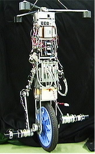
Figure 6 Robotic Unicycle model.

In the Off-Line stage a controlled object mathematical model is creating and the thermodynamic equations of its states are founding to calculate the entropy, which forming the GA’s fitness function and computer stochastic simulation with P(I)D controller parameters GA’s optimizer.

In the next stage the GA randomly selects an optimized PD’s controller parameters in the all possible solutions domain, using the minimum entropy production in the intelligent control system and in the complex nonlinear model dynamic behavior as a criterion for the solution suitability (fitness function). The fitness function of the GA is represented as:

$Eval=\min ((S^O-S^C)(\frac{d{S}^C}{dt}-\frac{d{S}^O}{dt}))$ (5.3)

where $\frac{d{S}^C}{dt}$ - is the control system's entropy production rate;$\frac{d{S}^O}{dt}$ - is entropy production rate in the motion of the robotic unicycle (Object) with following condition:$\frac{d{S}^C}{dt}>\frac{d{S}^O}{dt}$ . Description of entropy production rate calculation is presented in.^8,9

Thermodynamic equation of motion

The equations for entropy production rate calculation of the intelligent control system and dynamic motion of Robotic Unicycle are derived from approach as described in⁸These equations are described in the following form:

$\left[\begin{array}{c}\frac{d{S}^P}{dt}\\ \frac{d{S}^C}{dt}\end{array}\right]={\left[\begin{array}{cc}{M}_{i=j}(q)& 0\\ 0& 1\end{array}\right]}^{-1}\cdot \left[\begin{array}{c}{B}_{i=j}(q,\dot{q})\cdot {\dot{q}}^T(t)+D^T(\dot{q})\\ {\tau }_d^T\end{array}\right]\cdot {\dot{q}}^T(t)$ (5.4)

where: i,j=1..9; $M_{i=j}\left(q\right)$ is a 9X9 diagonal matrix of inertial acceleration’s terms $M\left(q\right)$ derived from Lagrange equations; $B_{i=j}(q,\dot{q})$ is a 9X9 diagonal matrix of Coriolis and centrifugal terms, derived from Lagrange equations; $D(\dot{q})$ is a 9-dimensional vector of viscous friction forces terms $D_i(\dot{q})=[D_1(\dot{q}),D_2(\dot{q}),D_3(\dot{q}),D_4(\dot{q}),D_5(\dot{q}),D_6(\dot{q}),D_7(\dot{q}),D_8(\dot{q}),D_9(\dot{q})]$ ; ${\tau }_d$ is a 9-dimensional vector of torque's dissipative parts $k{d}_i^{}\cdot [\dot{\beta },\dot{\gamma }]$ ,${\tau }_d=[0,{\tau }_3,{\tau }_{1,2},0,0,0,0,0,0]$ .

Following the Figure 3, the next step is the training of the control system based on the optimized controller parameters obtained from the GA and obtaining lookup tables (FC Knowledge Base) using the FNN.

In On-Line mode basing on the obtained lookup tables the P(I)D controller parameters of the robotic unicycle are changes by a fuzzy controller in real time.

⁴Sagawa T, Ueda M. Minimal Energy Cost for Thermodynamic Information Processing: Measurement and Information Erasure // Phys. Rev. Lett. – 2009. – Vol. 102. – No 25. – Pp. 250602.– Erratum. Phys. Rev. Lett. 106, 189901.– 2011.

⁵HorowitzJ. M., SandbergH. Second-law-like inequalities with information and their interpretations // New Journal of Physics. – 2014. – Vol. 16. – Pp. 125007.

Soft Computing Simulation structure in MathLab Simulink^® system is shown in Scheme 1. It consists from following parts:

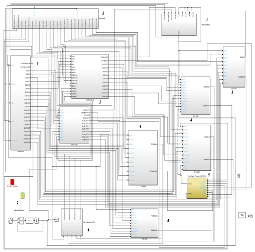
Scheme 1 MathLab Simulink^® diagram of the Robotic Unicycle computer simulation-main part.

1. Block of main equations;
2. Block of random excitation;
3. Blocks of equation's coefficients;
4. Blocks of Lagrangian multipliers calculation;
5. Block of Intelligent control system based on Soft Computing – GA or FNN.

In all simulation cases, the real parameters of the robotic unicycle model were used see the Figure 6, and the corresponding stochastic effects: disturbing from the floor to the yaw rotation angle and jamming in the closed-links mechanism. (Figure 7).

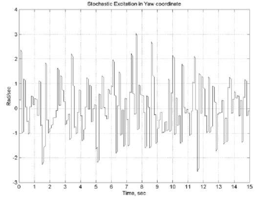
Figure 7 Simulated stochastic excitations - from a floor roughness’s and jamming in closed-links mechanisms.

The method of algebraic loops expulsion, described in detail in the patent,¹⁹ was applied to accelerate the simulation processes. This method allowed to accelerate the computer simulation process - integration expenses is decreases about 190 times with the difference in integration result less than 1%, as shown in Figure 8&9.

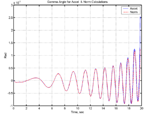
Figure 8 The accelerated and standard model’s an integrating accuracy example (with & without algebraic loops).

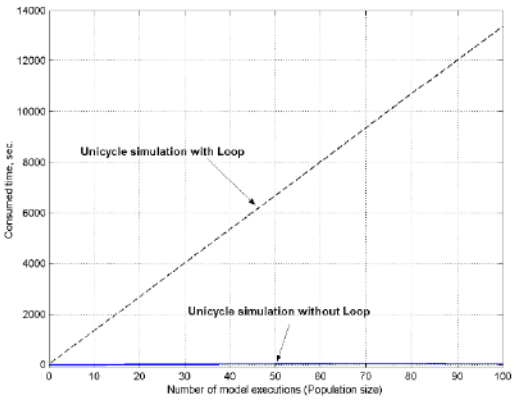
Figure 9 Integration time comparison for accelerated & standard models.

Simulation results discussion

In Figure 5 shown the comparison of three types of control approaches:

1. Conventional PD controller with fixed gain coefficients - temporal mechanical and thermodynamic controlled system behavior;
2. The GA with fitness function as minimum of entropy production rate for conventional PD controller.
3. The Fuzzy PD controller with lookup tables obtained after learning process by FNN with pattern from GA.

Such structure is the most applicable because of its flexibility, it has an opportunity to change only necessary separated blocks, such as control, main equations, excitation etc., without changing the whole structure.

From represented results it is visible, that:

1. usage of the approach described above, with application of a minimum entropy production rate as fitness function in GA and learning process by FNN, is completely justified;
2. dynamic motion occurs more smoothly even the control signal's discretization time is use in PD-GA and Fuzzy PD controllers with sampling time=0.05 sec.

Entropy production rate for the Pitch angle after the learning by FNN is decreased to 10 times. For the Yaw and Roll angles Entropy production rate is 10 times less for PD-GA and 1000 times less for the Fuzzy PD than for cconventional PD controller.

However, such energy transmitting increases amplitude of Pitch angle in case of PD-GA controller that conducts to increase torque in Links control system. But, after learning by FNN the motion in the pitch direction becomes smooth with small amplitude. It confirms about learnability and intellectualization of the Robotic Unicycle control system.

As can be seen from Figure 10, the movement of the model is smoother, which leads to a saving of the resource of the system as a whole. Also shown are the changes in the gain kp1, kd1, kp2, kd2 of the control equations (4.1) and (4.2). From the Figure 11 its visible that the model movement is going smoother, which leads to the system resource saving at whole. There are also shown the gain coefficients kp1, kd1, kp2, kd2 changes in the control equation (4.1) and (4.2).

Figure 10 Stochastic simulation results of Robotic Unicycle Model: Temporal mechanical and thermodynamic behavior of Robotic Unicycle with: a) conventional PD controller; b) PD-GA controllers; c) Fuzzy PD controllers; Temporal mechanical and thermodynamic behavior; d) conventional PD control system torques; e) PD-GA control system torques; f) Fuzzy PD control system torques.

Figure 11 Stochastic simulation results of Robotic Unicycle Model with different GA’s fitness functions Eval u Eval.

The introduction of the GA fitness function in the generalized function’s quadratic form is excluding the controls local instability (negative value of the generalized entropy). As a consequence, it gives improved characteristics of control quality (minimum complexity in the implementation of the gain coefficients changes by time, minimum driving mechanisms efforts and useful resource consumption). In this case, the information-thermodynamic law of the compromised distribution of the conflicting control qualities (stability, controllability and robustness) is fully implemented.

Experimental results discussion

Created in 1997-2000, the Cableless Robotic Unicycle is shown in Figure 6. The experimental results are represented in Figure 12–13. The time of the full-scale experiment was limited to 8 seconds due to the adverse effect of the gyroscopic sensors drift signal and low capacity of existed accumulators.

Figure 12 Experimental results, angles - pitch β, roll γ and yaw α angles.

Figure 13 Experimental results of the fuzzy gains temporal behavior kp1, kd2, kp2, kd2 for 2 PD controllers.

Though, it should be noted that sampling (more than 0.001 sec) of control signal from conventional PD, as it is present in real model, offers the Unicycle simulation system to "falling" after 8–10 sec.

In Figure 12 shows the experimental results for the cableless unicycle model. As it shown, the robot's lateral stability - in the roll direction $\gamma$ , and posture in the pitch direction $\beta$ is obtained.

In Figure 13 shown the temporal behavior of the fuzzy gains kp1, kd2, kp2, kd2 for 2 PD controllers (Eq. 4.1, 4.2).

From the result in Figure 12 is observed that the robot's posture in the yaw direction a is changed rapidly during the experiment, which indicates a satisfactory redistribution of control energy that provides lateral stability of the robot (roll $\gamma$ ) and tracking stochastic excitations on the model (floor roughness’s and jamming in closed-links mechanisms) by controlling the yaw angle $\alpha$ and pitch angle $\beta$ .

Remark 1: The obtained experimental results were achieved using empirically generated fuzzification and defuzzification for the gain coefficients kp1, kd2, kp2, kd2 of two fuzzy PD controllers, which were generated on the basis of preliminary results of GA simulation with the fitness function-reduction only the entropy production rate of the control system, i.e. incomplete simulation process of soft computing technology. The simulation results presented above were obtained later, upon completion of the Robotic Unicycle mathematical model development (Figure 4), (Eq. (1.2)), formation the soft computing process technology (Figure 2), and most importantly, the appearance of this approach calculating possibility-appropriate computational capabilities, without which this process was extremely difficult or impossible.

Remark 2: Despite of this, the obtained result at this time and with those computational capabilities, leads to confirmation of quite satisfactory operation of the represented structure of the intelligent control system. The represented structure of the process, as well as the new developments in this direction, is planned to be fully applied in the new prototype - an Autonomous Flexible Robotic Unicycle.

Related works: Emotional learning in the amygdala. In contrast to Figure 1, the system operation consists of two levels: the amygdale learns to predict and react to a given reinforcement signal. This subsystem cannot unlearn a connection. The incompatibility between predictions and the actual reinforcement signals causes inappropriate responses from the amygdala. As depicted in Figure 14, the system on Figure 14, consists of four main parts.²⁷ Sensory input signals first enter the thalamus. Since the thalamus must provide a fast response to stimuli, in this model the maximum over all stimuli S is sent directly to the amygdala as another input. The amygdala receives inputs from the thalamus and sensory cortex, while the orbitofrontal cortex (OFC) part receives inputs from the sensory cortex and the amygdala. The system also receives a reinforcing signal (REW – emotional signal).

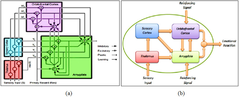
Figure 14 Graphical depiction of the brain emotional learning process (a) and the process of generating emotional reactions in the limbic part of human brain (b).

For each A node in the amygdala, there is a plastic connection weight V_i. Any input is multiplied by this weight to provide the output of the node. The O nodes show similar behavior, with a connection weight W_i applied to the input signal to create an output. There is one output node in common for all outputs of the model, called E (Figure 14). The E node sums the outputs from A except for the A_th and then subtracts the inhibitory outputs from the O nodes. The result is the output from the model.

The OFC learns to prevent the system output if such mismatches occur. The learning in the amygdala and the OFC is performed by updating the plastic connection weights, based on the received reinforcing and stimulus signals.

Example: Let us consider briefly Brain Emotional Learning Based Intelligent Controller (BELBIC) structure.²⁷ In a biological system, emotional reactions are utilized for fast decision‐making in complex environments or emergency situations. It is thought that the amygdala and the orbitofrontal cortex are the most important parts of the brain involved in emotional reactions and learning. The amygdala is a small structure in the medial temporal lobe of the brain that is thought to be responsible for the emotional evaluation of stimuli. This evaluation is in turn used as a basis for emotional states and reactions and is used for attention signals and laying down long‐term memories. The amygdala and the OFC compute their outputs based on the emotional signal (the reinforcing signal) received from the environment. The final output (the emotional reaction) is calculated by subtracting the amygdala’s output from the orbitofrontal cortex’s (OFC) output (Figure 14). A control system strategy, based on brain emotional learning, was proposed by Caro Lucas in the early 2000s (Lucas et al). The limbic model used was based on the neural link, between the amygdale and the orbitofrontal cortex, proposed by Balkenius and Moren. This control paradigm is commonly designated by BELBIC which stands for brain emotional learning based intelligent control. The reasoning behind the integration of the limbic model into a closed loop control system can be tracked down to the seemingly robust way that the brain performs decision making. Actually, control has all to do with decision making: the controller goal is to devise the best input actions based on the incoming information according to the system states. These actions can be taken considering the past, the present or even forecasts on the future system states. Hence the controller produces a mapping between its input signals and the output control signals by means of an arbitrary decision function which can be described by means of differential equations, as in PID-controllers, or by an inference mechanism such as in Fuzzy or Neuro-Fuzzy control. Alternatively it can be based on the result of the optimization of a cost function such as linear quadratic regulators (LQR) or model predictive control (MPC). In the BELBIC control system architecture this input-to-output transformation is imposed by means of the limbic system model. In this case, both the external stimuli and reward signals are generated in such a way as to produce a closed loop system response according to some target characteristics. In addition, due to the recursive nature of the weights update law, this controller is able to gradually learn how to handle changes in the system dynamics. A key point in BELBIC is the external stimulus and reward signals definition.

Notice that there are not universal rules to carry out this task. This choice is flexible and must be custom defined according to the end application. For example in Lucas et al. the reward signal r(t) is obtained as a weighted sum of the error signal and the control effort and the external stimulus signal i(t) is defined as a linear combination of the system output and its first derivative.

It should be observed that it essentially converts two sets of inputs (sensory inputs and emotional cues or reinforcing signals) into the decision signal (the emotional reaction) as its output. Closed loop configurations using this block (BELBIC) in the feedforward control loop of the total system in an appropriate manner have been implemented so that the input signals have the proper interpretations. The block implicitly implemented the critic, the learning algorithm and the action selection mechanism used in the functional implementations of emotionally based (or, generally, reinforcement learning based) controllers, all at the same time.

Reza Keramat, et al¹⁵ consider that in practical systems important information originates from two sources. One of the sources is the experts, who define their knowledge of the system using the natural language. The other consists of measurements and mathematical models derived from physical laws. Hence, what matters is how to incorporate these types of information into the design of systems. The question is that how it is possible to formulate human knowledge within a framework similar to mathematical models.

In other words, the main question is “How is it possible to convert human knowledge to a mathematical formula?”

Basically, the main function of a fuzzy system is to make such a conversion possible. Fuzzy systems are based on knowledge or rules. The core of a fuzzy system is a knowledge base following the IF-THEN fuzzy rules. If a fuzzy system is used by a controller, the controller is called “fuzzy controller”.

The fuzzy controller designed for the full bridge DC-DC converter takes two inputs: error ($e$ ) and error variations ($\Delta e$ ). The membership input functions for this controller are in the range of [-5 , 5]. Membership functions for each of the two input components of error and error variations are shown in Figure 15.

Figure 15 The membership functions for e and Δe.

Seven membership functions are used here for the input: negative big (NB), negative medium (NM), negative small (NS), zero (Z), positive big (PB), positive medium (PM), and positive small (PS).The controller output is assumed to be equal to the duty cycle, which varies between 0 and 0.5. Figure 16 displays the controller output functions.

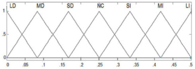
Figure 16 The output membership functions.

Reza Keramat, et al¹⁵ show the effectiveness of BELBIC for the full bridge DC-DC converter. Figure 17 shows the system output voltage after the application of the fuzzy and BELBIC controllers. As seen in this figure, the BELBIC has a slight overshoot while the fuzzy controller has a considerable overshoot (the initial overshoot is 35 V). The time required for stabilization is almost the same in both cases. It is therefore concluded that the BELBIC outperforms the fuzzy controller.

Figure 17 The comparison of the fuzzy controller with the BELBIC.

In¹⁵ experiment the BELBIC controller outperforms the fuzzy controller. Considering the uncertainty of system parameters (including inductance, capacitance, and input voltage and acceptable variations of load), the BELBIC presents better performance than the fuzzy controller. Although fuzzy control is a robust and effective method for a large number of engineering systems, but its design (and consequently its performance) is almost depend on the experience and tact of the designer. Furthermore, after design and installation, its performance is not improved, and in other word, it is not a learning-based or intelligent controller.

It can be stated that a Learning Based Intelligent Control which 'may' in the first step, act not as satisfying as any another modern controller, any straight-forward-designed controller after a few iterations thanks to its learning automata feature. Based on this deduction, we felt no need to emphasize the comparison of these controllers after setting optimization.

This work represents the basic idea of intelligent control of dynamical, globally unstable, nonlinear objects on the example of Robotic Unicycle. The basis of this approach is a qualitative physical analysis of the robot dynamic movement with the introduction of intelligent feedback in the control system and the implementation of instinct and intuition mechanisms based on the FNN and GA.

The main components of an intelligent control system based on soft computing and robustness determination are also represented. Thus, there is an adaptation of the two fuzzy PD controllers’ parameters to achieve a stable motion of the robotic unicycle over a long (finite) time interval, without changing the structure of the control system executive level, is achieved.^16–19

The introduction of these two new mechanisms to an intelligent control system is based on the principle of minimum entropy production in the robot unicycle's motion and the control system itself. The fuzzy stochastic simulation of thermodynamic equations of motion and the intelligent control system confirm the effectiveness of the robot's postural stability control to handle the system's nonlinearity.^20–22

In this case the unicycle robot model is a new benchmark for intelligent fuzzy controlled motion of a nonlinear dynamic system with two (local and global) 3D unstable states.

Use of a fuzzy gain schedule PD controller with look-up tables calculated by FNN, offers the ability to use instinct and intuition mechanisms in on line to intellectualize the intelligent control system levels.

Quantum soft computational intelligence toolkit^23–26 applied to design of self-organized conventional PD controllers can increase the robustness of robotic unicycle.^27–29

None.

None.

The authors declare that there was no conflict of interest.

1. Schoonwinkel A. Design and test of a computer stabilized unicycle. A Dissertation submitted to the department of aeronautics and astronautics and the committee on graduate studies. USA: Stanford University;1987.
2. David William V. Nonlinear control of an autonomous unicycle robot: practical issues.A Dissertation submitted to the department of aeronautics and astronautics. USA: Massachusetts Institute of Technology; 1992.
3. Ulyanov SV, Sheng ZQ,Yamafuji K. Fuzzy Intelligent control of robotic unicycle: A New benchmark in nonlinear mechanics. Proc. Intern. Conf. on Recent Advanced Mechatronics; Istanbul, Turkey; 1995.
4. Ulyanov SV, Sheng ZQ, Yamafuji K.et al. Self-organization fuzzy chaos intelligent controller for a robotic unicycle: A New benchmark in AI control. Proc. of 5th Intelligent System Symposium: Fuzzy, AI and Neural Network Applications Technologies; Tokyo;1995.
5. Sheng ZQ, Yamafuji K,Ulyanov SV. Study on the Stability and Motion Control of a Unicycle : 4th Report, Fuzzy Gain Schedule PD Controller for Managing Nonlinearity of System.JSME international journal. Ser. C, Dynamics, control, robotics, design and manufacturing.1996;39(3):569–576.
6. Panfilov SA, Ulyanov VS, Litvintseva LV, et al. Robust Fuzzy Control of Non-Linear Dynamic Systems Based on Soft Computing with Minimum of Entropy Production Rate. Proc. Int. Conf. ICAFS; 2000; Siegen, Germany;2000.
7. Rouch N, Habets P,Laloy M. Stability Theory by Liapunov's Direct Method. Berlin: Springer; 1977.
8. Ulyanov VS,PanfilovSA, Ulyanov SV. Principle of minimum entropy production in applied soft computing for advanced intelligent robotics and mechatronics. Soft Computing. 2000;4(3):141–146.
9. Ulyanov VS, Yamafuji K, Ulyanov SV, et al. Computational intelligence with new physical controllability measure for robust control algorithms of extension-cableless robotic unicycle.Journal of Advanced Computational Intelligence.1999;3(2):136–147.
10. Ulyanov SV,Yamafuji K. Fuzzy Intelligent emotion and instinct control of a robotic unicycle.Proceedings of 4th IEEE International Workshop on Advanced Motion Control - AMC '96 - MIE; 1996 Mar 18–21; Mie, Japan; 1996.
11. Ulyanov SV, Watanabe S, Yamafuji K,et al. A new physical measure for mechanical controllability and intelligent control of a robotic unicycle on basis of intuition, instinct and emotion computing. Proc. 2nd Intern. Conf. on Application on Fuzzy Systems and Soft Computing (ICAF’96); Siegen, Germany;1996. p. 49–58.
12. Ulyanov SV, Watanabe S, Ulyanov VS, et al.Soft computing for the intelligent control of a robot unicycle based on a new physical measure for mechanical controllability.Soft Computing. 1998;2(2):73–88.
13. Lauk M, Chow CC, Pavlik AE, et al. Human balance out of equilibrium: Non-equilibrium statistical mechanics in posture control. Physical Review Letters. 1998;80(2).
14. Ulyanov SV, Yamafuji K, Ulyanov VS, et.al. Computational intelligence for robust control algorithms of complex dynamic systems with minimum entropy production.Journal of Advanced Computational Intelligence. 1999;3(2):82–98.
15. Keramat R, Ershadi M, Shojaeian S. A Comparison of Fuzzy and Brain Emotional Learning-Based Intelligent Control Approaches for a Full Bridge DC-DC Converter. International Journal of Industrial Electronics, Control and Optimization. 2019;2(3):197–206.
16. Murata girl. Murata innovator in electronics. Japan; 2011.
17. Wieser E. Machine learning for a miniature robotic unicycle. Master of science thesis of Cambridge University. UK; 2017.
18. De Vries JF. Redesign & implementation of a moment exchange unicycle robot. Master of science thesis of Twente University. Netherlands; 2018.
19. Kim S, Lee J, Hwang J, et al. Dynamic modeling and performance improvement of a unicycle robot. J Instit of Control Robotics and Systems.2010;16(11):1074–1081.
20. Ulyanov SV, Sergei P.System and method for simulation of nonlinear dynamic systems applicable within soft computing. USA Patent Application Publication. 2004
21. Sergey AP, Ludmila VA, Ulyanov SV. Soft computing optimizer of intelligent control systemsDesign: The Structure And Applications.2005
22. Ulyanov SV. System for soft computing simulation. 2006.
23. Ulyanov SV. Soft computing optimizer of intelligent control system structures. 2005.
24. Ulyanov SV. System and method for control using quantum soft computing.2001.
25. Sergey AP, Sergey VU. Efficient simulation system of quantum algorithm gates on classical computer based on fast algorithm. 2006.
26. Litvintseva LV, Ulyanov IS, Ulyanov SV, et al. Quantum fuzzy inference for knowledge base design in robust intelligent controllers.J. of Computer and Systems Sciences Intern. 2007;46(6):908–961.
27. Ulyanov SV.Self-organizing quantum robust control methods and systems for situations with uncertainty and risk. 2014.
28. Ulyanov SV. Quantum fast algorithm computational intelligence PT I:SW / HW Smart toolkit. Artificial Intelligence Advances. 2019;1(1):18–43.
29. Beheshti Z, Zaiton S, Hashim M. A Review of Emotional Learning And It’s Utilization in Control Engineering.Int. J. Advance. Soft Comput. Appl.2010;2(2):2074–8523.