A wolf-moose predator-prey system is defined as a nonlinear continuous time differential equation system. The parameters are estimated via a discretized approximation and empirical data from Isle Royale, USA, representing a 61 year period. All parameter estimates confirm the hypotheses and all P-values are below 5%. Possible dynamic equilibria are determined as explicit general functions of the parameters and as numerical values based on the empirical data. General dynamic properties of the system are determined via phase -plane analysis and nonlinear simulation. The nonlinear system is also linearized close to the single equilibrium with two strictly positive populations. The explicit equations of the time path of the linearized system are compared to the nonlinear simulation. Both methods give almost identical solutions close to the equilibrium. Far from the equilibrium, the time paths of the two methods deviate considerably. The solution is a stable converging spiral (center) (unstable diverging spiral) in case the system equilibrium prey population is located at a higher (the same) (lower) level than the population level that gives maximum sustainable net production. Based on the empirically determined expected parameter values, the system is stable but converges very slowly, as a spiral, to the two-species equilibrium. The estimated standard deviations of the parameters can be used to determine the probability that the system solution is a center or an unstable diverging spiral. The optimal management of the wolf-moose system is also determined via sustainable optimal control. Moose hunting and adjustments of the wolf population based on different prices and values of sustainable population levels are derived. Optimal hunting and stock levels are determined and reported as explicit functions of all parameters and prices.

Keywords: predator prey system, dynamics, stability, differential equation system, linearization, economic optimization, sustainable control

Predator prey systems have gained considerable interest ever since the pioneering work by Lotka and Volterra, described in Lotka.¹ In books on differential equations and applications, several authors have devoted many pages to the inspiring problems of predator prey systems. Some of the most well written cases are found in Braun,² Blanchard et al.,³ & Tung.⁴ In this study, the ambition is to investigate the dynamic properties of a typical predator prey system, namely the wolf-moose system. Such systems are frequent in large parts of the world, in the large forests in North America, Russian Federation and the Nordic countries. On a rather isolated island, Isle Royale, in Lake Superior, USA, the conditions are favorable for the study of such a system. Detailed data covering the populations of wolf, moose and several other variables of potential interest, have been gathered there since the year 1959. The empirical data used in this study are found in Appendix 1, and come from Michigan Tech.⁵ Some earlier time series and simulations connected to the Isle Royale project have been presented by Knadler.⁶ When we consider predator prey systems, this may be done with different objectives. First, the system may be considered as more or less “natural” and unaffected by human regulation. In the first part of this paper, this is done. The dynamic properties of the “unregulated” system are analyzed and considerable attention is given to equilibria and stability. Second, we may also investigate if and how the system may be controlled, in order to satisfy some interests. In the second part of this paper, the options to hunt for moose and to regulate the wolf population, will be used as control variables. An objective function will be defined, where the profits from the hunting and the valuation of the wolf population will be considered. We will see how the optimal management can be designed in a way that makes the objective function and the animal populations sustainable, and simultaneously maximizes the selected objective function.

Motivation for the differential equations

In alternative predator prey models, the details of the differential equations can differ in several ways. In this paper, particular functional forms of relevance to the species under study will be assumed and empirically tested. W denotes the size of the wolf population. In equation (1), we see how the relative growth of the wolf population depends on M, the size of the moose population and the two parameters g and h. The logic behind the equation is that g is the rate of death. The relative reproduction of the wolf is assumed to be an increasing function of the moose population.

$\left(W>0\right)\Rightarrow \frac{\stackrel{•}{W}}{W}=\frac{\left(\frac{dW}{dt}\right)}{W}=-g+hM$   (1)

The functional form of equation (1) is linear. No nonlinear dependences can be discovered via residual analysis. Hence, the linear function is selected. In case the number of wolfs is zero, there is no predation. Then, equation (2) shows that the relative growth of the moose population is a decreasing function of the moose population. The two parameters a and b are strictly positive.

$(W=0)\Rightarrow \frac{\stackrel{•}{M}}{M}=\frac{\left(\frac{dM}{dt}\right)}{M}=a-bM$   (2)

Equation (3) follows from (2) and says that, without predation, the moose population growth is a strictly concave function of the population level. This is also the basic assumption that is used in the logistic growth models with one species.

$(W=0)\Rightarrow \stackrel{•}{{\displaystyle M}}=aM-b{M}^2$   (3)

If the wolf population is strictly positive, they will survive by eating moose. Then, the moose population dynamics is modified, as we see in equation (4). The parameter c is strictly positive, representing the number of moose killed per year per wolf.

$(W>0)\Rightarrow \stackrel{{}_{•}}{M}=aM-b{M}^2-cW$   (4)

With the motivated differential equations, we obtain the simultaneous system (5).

$\{\begin{array}{cc}\stackrel{{}_{•}}{M}=& aM-b{M}^2-cW\\ \stackrel{•}{W}=& -gW+hMW\end{array}$   (5)

Empirical estimation of the differential equations

The two differential equations are approximated as two difference equations. The unit of time is years. The available empirical data set includes one pair of observations $(M,W)$ each year. $\Delta t=1$ .

$\{\begin{array}{cc}\stackrel{•}{M}\approx \frac{\Delta M}{\Delta t}=& aM-b{M}^2-cW\\ \stackrel{•}{W}\approx \frac{\Delta W}{\Delta t}=& -gW+hMW\end{array}$   (6)

Then, two multiple regression analyses were performed. The residuals $\left({\epsilon }_M,{\epsilon }_W\right)$ are assumed to be Normally distributed with zero means and correlations.

$\{\begin{array}{cc}\frac{\left(\frac{\Delta M}{\Delta t}\right)}{M}=& a-bM-c\frac{W}{M}+{\epsilon }_M\\ \frac{\left(\frac{\Delta W}{\Delta t}\right)}{W}=& -g+hM+{\epsilon }_W\end{array}$   (7)

M-regression

$\frac{\left(\frac{\Delta M}{\Delta t}\right)}{M}=0.372-0.178\frac{M}{1000}-6.593\frac{W}{M}+{\epsilon }_M$   (8)

${\epsilon }_M\sim N\left({\mu }_M,{\sigma }_M^2\right),{\mu }_M=0,{\sigma }_M\approx 0.174$   (9)

$\left(\frac{\Delta M}{\Delta t}\right)=0.372M-0.178\times {10}^{-3}{M}^2-6.593W+M{\epsilon }_M$   (10)

The number of observations was 60 and the multiple R value was 0.367. Clearly, since there is a second order term in the difference equation, the expected value of the difference is in general not constant over time. However, close to a dynamic equilibrium, for short time intervals, second order effects are very small and may be neglected.

$E\left(\stackrel{{}_{•}}{M}\right)\approx 0.372M-0.178\times {10}^{-3}{M}^2-6.593W$   (11)

W-regression

$\frac{\left(\frac{\Delta W}{\Delta t}\right)}{W}=-0.244+0.230\frac{M}{1000}+{\epsilon }_W$   (12)

${\epsilon }_W\sim N\left({\mu }_W,{\sigma }_W^2\right),{\mu }_W=0,{\sigma }_W\approx 0.334$   (13)

$\left(\frac{\Delta W}{\Delta t}\right)=-0.244W+0.230\times {10}^{-3}MW+W{\epsilon }_W$   (14)

The number of observations was 60 and the multiple R value was 0.272.

$E\left(\stackrel{{}_{•}}{W}\right)\approx -0.244W+0.230\times {10}^{-3}MW$   (15)

In Table 1, it is interesting to observe that all parameter values obtained the expected signs. Furthermore, they are all, with more than 95% probability, different from zero. The standard deviations of the parameters, found in Table 1, are important, partly because they can be used to estimate the probability that the differential equation system is stable. Later in this paper, it turns out that the system is stable in case the parameters really have the estimated expected values found in Table 1. If the deviations from these values are sufficiently large, the system may become unstable. Now, let us investigate the behavior of the approximated differential equation system. We make the following assumption:

$\left(\stackrel{{}_{•}}{M},\stackrel{{}_{•}}{W}\right)\approx \left(E\left(\stackrel{{}_{•}}{M}\right),E\left(\stackrel{{}_{•}}{W}\right)\right)$   (16)

The simplified estimated differential equation system is:

$\{\begin{array}{cc}\stackrel{{}_{•}}{M}=& 0.372M-0.178\times {10}^{-3}{M}^2-6.593W\\ \stackrel{{}_{•}}{W}=& -0.244W+0.230\times {10}^{-3}MW\end{array}$   (17)

Equilibria

The estimated differential equation system has several equilibria. We may consider the cases where both species have strictly positive population sizes, and where one or two of them are zero. Since the main interest in this paper concerns the two species situation, we start with Equilibrium 1.

Equilibrium 1

In equilibrium 1, we have $\left(M>0,W>0\right)$ .

Equation (18) shows that the moose population can be determined from the fact that the wolf population is in equilibrium.

$\left(W>0\wedge \stackrel{{}_{•}}{W}=0\right)\Rightarrow \left(0.230\times {10}^{-3}M=0.244\right)$   (18)

denotes the moose population in system equilibrium with a strictly positive value of the wolf population.

$\left(W>0\wedge \stackrel{{}_{•}}{W}=0\right)\Rightarrow \left(M\approx 1061\right)\Rightarrow \left(M_1\approx 1061\right)$   (19)

When the equilibrium moose population is known, we can use this in the moose growth equation, as we see in equation (20). From this, we can determine the equilibrium wolf population.

$\stackrel{{}_{•}}{M}=0.372M_1-0.178\times {10}^{-3}{M}_1{}^2-6.593W=0$   (20)

$6.593W=0.372M_1-0.178\times {10}^{-3}{M}_1{}^2$   (21)

$W=\frac{\left(0.372M_1-0.178\times {10}^{-3}{M}_1{}^2\right)}{6.593}$   (22)

$W_1$ denotes the wolf population in system equilibrium with strictly positive values of the moose and wolf populations.

$W_1=\frac{\left(0.372M_1-0.178\times {10}^{-3}{M}_1{}^2\right)}{6.593}\approx 29.47$   (23)

Equilibrium 2

In the absence of wolves, we can instantly determine the equilibrium moose population via equation (24).

$\left(M>0,W=0,\stackrel{{}_{•}}{M}=0\right)\Rightarrow \left(0.372M-0.178\times {10}^{-3}{M}^2=0\right)$   (24)

$0.372-0.178\times {10}^{-3}M=0$   (25)

$M_2$ denotes the moose population in system equilibrium without a wolf population.

$M_2\approx 2090$   (26)

Obviously, the equilibrium moose population is much lower in case there is a wolf population than if there are no predators in the forest. Of course, this also affects the environment, via more damages on the plants and trees that are eaten by moose.

Equilibrium 3

Here, we consider the maximum equilibrium growth (or “production”, the number of moose per year) of a moose population without any wolf population. This may represent a maximum desired by human moose hunters.

$\underset{M}{\max }Z=0.372M-0.178\times {10}^{-3}{M}^2$   (27)

First order optimum condition is:

$\frac{dZ}{dM}=0.372-2\cdot 0.178\times {10}^{-3}M=0$   (28)

There is one and only one optimal solution, namely:

$M_3\approx 1045$   (29)

The second order maximum condition is satisfied.

$\frac{d^{2}Z}{d{M}^2}=-2\cdot 0.178\times {10}^{-3}<0$   (30)

Hence the unique maximum of the equilibrium number of moose, continuously removed from the forest by hunters, is found in equation (31).

$Z^{*}\approx 194.36$   (31)

Qualitative analysis of the system dynamics

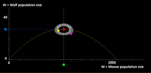
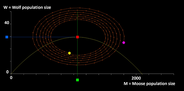
A phase plane is a visual display of certain properties of differential equations. In phase plane analysis, we investigate the dynamic properties of the solutions. Figure 1 shows the phase plane of the differential equation system. Along the curved strictly concave line, the moose population is in equilibrium. Along the vertical line, the wolf population is in equilibrium. The red box marks the most interesting Equilibrium 1. The equilibrium moose population and the equilibrium wolf populations are marked with green and blue boxes. The same notation is used in Figures 2–7. The “direction field” is indicated via arrows. The arrows show how the system moves over time. Clearly, the solutions will be spirals. The Figures 2 & 3 will confirm this conclusion.

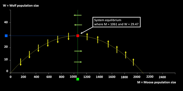
Figure 1 The phase plane of the system.

Figure 2 The time path of the populations close to the equilibrium, derived via the nonlinear differential equations in the differential equation system. The initial conditions, (M,W)=(1200,25), are marked by a purple ball and the terminal conditions are marked by a yellow ball. The total simulation time represents 200 years. Each year is marked by a small white ball.

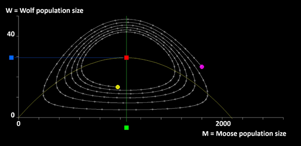
Figure 3 The time path of the populations far from the equilibrium, derived via the nonlinear differential equations in the differential equation system. The initial conditions, (M,W)=(1800,25), are marked by a purple ball and the terminal conditions are marked by a yellow ball. The total simulation time represents 200 years. Each year is marked by a small white ball.

Nonlinear simulation of the differential equation system

We may use the differential equation system (17) and simulate it with different initial conditions, to see how it develops. We use very short time intervals and determine the changes of the populations. Figures 2 & 3 show the results of such simulations with different initial conditions. The software used to create these graphs is found in Appendix 2. In the simulations, 20 000 short linear moves of both species are made over time intervals representing 0.01 year. The total time represents 200 years. We note that the solutions are very slowly converging spirals. Hence, the equilibrium seems to be a “sink”. Later, we will confirm this conjecture via a formal investigation of a linearized approximation of the system performed at the equilibrium. 

Linearization of the system close to equilibrium 1

Now, the system will be linearized close to Equilibrium 1. This is done primarily to formally determine if the solution converges, stays at a constant distance from, or diverges from the equilibrium. We will also be able to understand, in general, how the answer to this question depends on the parameters. Our system is found in (32).

$\{\begin{array}{cc}\stackrel{{}_{•}}{M}=& aM-b{M}^2-cW\\ \stackrel{{}_{•}}{W}=& -gW+hMW\end{array}$   (32)

In equilibrium, we have:

$\{\begin{array}{cc}\stackrel{{}_{•}}{M}=& a{M}_1-b{M}_1{}^2-c{W}_1=0\\ \stackrel{{}_{•}}{W}=& -g{W}_1+h{M}_1{W}_1=0\end{array}$   (33)

Now, we will let u and v represent small deviations from the equilibrium.

$M=M_1+u$   (34)

$W=W_1+v$   (35)

The differential equation system may now be rewritten as (36).

$\{\begin{array}{cc}\stackrel{{}_{•}}{M}=& a\left(M_1+u\right)-b{\left(M_1+u\right)}^2-c\left(W_1+v\right)\\ \stackrel{{}_{•}}{W}=& -g\left(W_1+v\right)+h\left(M_1+u\right)\left(W_1+v\right)\end{array}$   (36)

The system (37) follows:

$\{\begin{array}{cc}\stackrel{{}_{•}}{M}=& a{M}_1+au-b{M}_1{}^2-2b{M}_{1}u-b{u}^2-c{W}_1-cv\\ \stackrel{{}_{•}}{W}=& -g{W}_1-gv+h{M}_1{W}_1+h{M}_{1}v+h{W}_{1}u+huv\end{array}$   (37)

Thanks to the fact that we have an equilibrium, we get (38). This is further developed into (39) and (40).

$\left(\{\begin{array}{c}a{M}_1-b{M}_1{}^2-c{W}_1=0\\ -g{W}_1+h{M}_1{W}_1=0\end{array}\right)\Rightarrow \{\begin{array}{cc}\stackrel{{}_{•}}{M}=& au-2b{M}_{1}u-b{u}^2{}_1-cv\\ \stackrel{{}_{•}}{W}=& -gv+h{M}_{1}v+h{W}_{1}u+huv\end{array}$   (38)

$\{\begin{array}{cc}\stackrel{{}_{•}}{u}=\stackrel{{}_{•}}{M}=& au-2b{M}_{1}u-b{u}^2{}_1-cv\\ \stackrel{{}_{•}}{v}=\stackrel{{}_{•}}{W}=& -gv+h{M}_{1}v+h{W}_{1}u+huv\end{array}$   (39)

$\{\begin{array}{cc}\stackrel{{}_{•}}{u}=& \left(a-2b{M}_1\right)u+\left(-c\right)v-b{u}^2\\ \stackrel{{}_{•}}{v}=& \left(h{W}_1\right)u+\left(-g+h{M}_1\right)v+huv\end{array}$   (40)

As we approach an equilibrium, the second order terms go to zero much faster than the first order terms.

$\left(u\to 0\wedge v\to 0\right)\Rightarrow \left(\frac{u^2}{u}\to 0\wedge \frac{uv}{u}\to 0\wedge \frac{uv}{v}\to 0\right)$   (41)

Hence, close to the equilibrium, $u^2\approx 0\wedge uv\approx 0$ .

$\{\begin{array}{cc}\stackrel{{}_{•}}{u}=& \left(a-2b{M}_1\right)u+\left(-c\right)v\\ \stackrel{{}_{•}}{v}=& \left(h{W}_1\right)u+\left(-g+h{M}_1\right)v\end{array}$   (42)

We may express the linear differential equation system as (43).

$\left[\begin{array}{c}\stackrel{{}_{•}}{u}\\ \stackrel{•}{v}\end{array}\right]=\left[\begin{array}{cc}\left(a-2b{M}_1\right)& -c\\ h{W}_1& \left(-g+h{M}_1\right)\end{array}\right]\left[\begin{array}{c}u\\ v\end{array}\right]$   (43)

We remember that the wolf population is in equilibrium. This gives (44).

$\left(\stackrel{{}_{•}}{W}=0\right)\Rightarrow \left(-g+h{M}_1\right)=0$   (44)

Hence, the differential equation system is simplified.

$\left[\begin{array}{c}\stackrel{{}_{•}}{u}\\ \stackrel{{}_{•}}{v}\end{array}\right]=\left[\begin{array}{cc}\left(a-2b{M}_1\right)& -c\\ h{W}_1& 0\end{array}\right]\left[\begin{array}{c}u\\ v\end{array}\right]$   (45)

The parameter values that we now need are these:

$a=0.372,b=0.178\times {10}^{-3},c=6.593,g=0.244,h=0.230\times {10}^{-3},M_1\approx 1061,W_1\approx 29.47$   (46)

With the parameter values, we get:

$\left[\begin{array}{c}\stackrel{•}{u}\\ \stackrel{•}{v}\end{array}\right]=\left[\begin{array}{cc}-5.716\times {10}^{-3}& -6.593\\ 6.778\times {10}^{-3}& 0\end{array}\right]\left[\begin{array}{c}u\\ v\end{array}\right]$   (47)

We consider exponential functional forms, as in (48).

$u(t)=u_0{e}^{\lambda t}\wedge v(t)=v_0{e}^{\lambda t}$   (48)

Then, the time derivatives can be obtained and included in the equations, as in (49).

$\left[\begin{array}{c}\lambda u\\ \lambda v\end{array}\right]=\left[\begin{array}{cc}-5.716\times {10}^{-3}& -6.593\\ 6.778\times {10}^{-3}& 0\end{array}\right]\left[\begin{array}{c}u\\ v\end{array}\right]$   (49)

Clearly, it is necessary that (50) is satisfied.

$\left[\begin{array}{cc}\left(-5.716\times {10}^{-3}-\lambda \right)& -6.593\\ 6.778\times {10}^{-3}& \left(0-\lambda \right)\end{array}\right]\left[\begin{array}{c}u\\ v\end{array}\right]=\left[\begin{array}{c}0\\ 0\end{array}\right]$   (50)

We want to be sure that nontrivial solutions can be obtained. This implies the condition found in (51).

$\left(u\ne 0\wedge v\ne 0\right)\Rightarrow \left(\left|D\right|=\left|\begin{array}{cc}\left(-5.716\times {10}^{-3}-\lambda \right)& -6.593\\ 6.778\times {10}^{-3}& \left(0-\lambda \right)\end{array}\right|=0\right)$   (51)

Hence, a quadratic equation has to be solved. This is found in (52).

$\left|D\right|={\lambda }^2+5.716\times {10}^{-3}\lambda +44.687\times {10}^{-3}=0$   (52)

$\left|D\right|={\lambda }^2+p\lambda +q=0$   (53)

There are, in general, two solutions.

$\lambda =-\frac{p}{2}\raisebox{1ex}{$+$}\!\left/ \!\raisebox{-1ex}{$-$}\right.\sqrt{{\left(\frac{p}{2}\right)}^2-q}$   (54)

$\lambda =-0.002858\raisebox{1ex}{$+$}\!\left/ \!\raisebox{-1ex}{$-$}\right.\sqrt{-0.0446788}$   (55)

Obviously, we have two complex roots. The real part is negative. This means that the solutions will be converging spirals. Since the real part is close to zero, the solution converges very slowly. In fact, it takes approximately 243 years for the spiral to get 50% closer to the equilibrium. This seems reasonable if we compare the spirals in the Figures 2 & 3.

$\lambda =-0.002858\raisebox{1ex}{$+$}\!\left/ \!\raisebox{-1ex}{$-$}\right.0.21137i$   (56)

$\varphi =-0.002858,\psi =0.21137$   (57)

In order to simplify and generalize the notation in the following section, we use equation (58).

$\lambda =\varphi \raisebox{1ex}{$+$}\!\left/ \!\raisebox{-1ex}{$-$}\right.\psi i$   (58)

The equations (59) to (65) show the steps of analysis until we end up with the system solution, found in equation (66).

$u=e^{\varphi t}\left(A\cos \left(\psi t\right)+B\sin \left(\psi t\right)\right)$   (59)

$\stackrel{{}_{·}}{u}=\varphi e^{\varphi t}\left(A\cos \left(\psi t\right)+B\sin \left(\psi t\right)\right)+e^{\varphi t}\left(-\psi A\sin \left(\psi t\right)+\psi B\cos \left(\psi t\right)\right)$   (60)

$\stackrel{{}_{·}}{u}=e^{\varphi t}\left(\left(\varphi A+\psi B\right)\cos \left(\psi t\right)+\left(\varphi B-\psi A\right)\sin \left(\psi t\right)\right)$   (61)

$\gamma =-0.005716,\Omega =-6.593$   (62)

$\stackrel{{}_{·}}{u}=\gamma u+\Omega v$   (63)

$v=\frac{\stackrel{{}_{·}}{u}-\gamma u}{\Omega }$   (64)

$v=\frac{1}{\Omega }{e}^{\varphi t}\left(\left(\varphi A+\psi B-\gamma A\right)\cos \left(\psi t\right)+\left(\varphi B-\psi A-\gamma B\right)\sin \left(\psi t\right)\right)$   (65)

$\{\begin{array}{cc}u(t)=& e^{\varphi t}\left(A\cos \left(\psi t\right)+B\sin \left(\psi t\right)\right)\\ v(t)=& \frac{1}{\Omega }{e}^{\varphi t}\left(\left(\left(\varphi -\gamma \right)A+\psi B\right)\cos \left(\psi t\right)+\left(\left(\varphi -\gamma \right)B-\psi A\right)\sin \left(\psi t\right)\right)\end{array}$   (66)

Parameter determination

Now, via equation (66), the parameters of the linear approximation can be determined.

At time zero, we have:

$\{\begin{array}{c}u(0)=A\\ v(0)=\frac{1}{\Omega }\left(\left(\varphi -\gamma \right)A+\psi B\right)\end{array}$   (67)

$A=u(0)$   (68)

$B=\frac{\Omega v(0)+\left(\gamma -\varphi \right)A}{\psi }$   (69)

The initial conditions that were also used in the simulation close to the equilibrium, illustrated in Figure 2, are applied:

$\left(M_0,W_0\right)=\left(1200,25\right)$   (70)

After the derivations shown via equations (71) to (75), all parameters of the linear approximation of the system path will be known.

$\{\begin{array}{c}u(0)=M_0-M_1\\ v(0)=W_0-W_1\end{array}$   (71)

$\{\begin{array}{c}u(0)=1200-1061\\ v(0)=25-29.47\end{array}$   (72)

$\{\begin{array}{c}u(0)=139\\ v(0)=-4.47\end{array}$   (73)

$A=u(0)=139$   (74)

$B=-31.192v(0)-0.013521A=137.55$   (75)

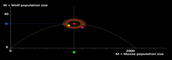
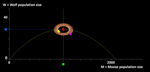
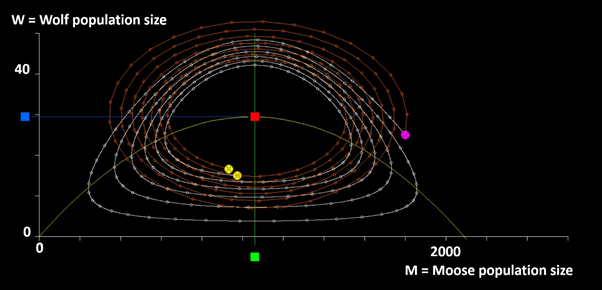
Now, the linear approximation of the system can be studied. The numerical derivations are found in the software included in Appendix 2. In Figure 4, we see how the linear approximation of the differential equation system works close to the equilibrium. In Figure 5, the time path of the linear approximation is compared to the time path of the original nonlinear differential equation system solution. We note that the linear approximation works very well close to the equilibrium. As the distance to the equilibrium increases, the reliability of the linear approximation is reduced.

Figure 4 The time path of the populations close to the equilibrium, derived via the time path of the linear approximation of the differential equation system. The initial conditions, (M,W)=(1200,25), are marked by a purple ball and the terminal conditions are marked by a yellow ball. The total simulation time represents 200 years. Each year is marked by a small orange ball.

Figure 5 Comparison of the time paths close to the equilibrium, via the nonlinear simulation (white path) and the solution to the linear approximation (orange path). The initial conditions, (M,W)=(1200,25), are marked by a purple ball and the terminal conditions are marked by yellow balls. The total simulation time represents 200 years. Each year is marked by small white and orange balls. Both time paths start in the same point and end in almost the same point, 200 years later. The two solutions stay close all the time. The linear approximation is reliable close to the equilibrium.

Figure 6 The time path of the populations far from the equilibrium, derived via the time path of the linear approximation of the differential equation system. The initial conditions, (M,W)=(1800,25), are marked by a purple ball and the terminal conditions are marked by a yellow ball. The total simulation time represents 200 years. Each year is marked by a small orange ball.

Figure 7 Comparison of the time paths far from the equilibrium, via the nonlinear simulation (white path) and the solution to the linear approximation (orange path). The initial conditions, (M,W)=(1800,25), are marked by a purple ball and the terminal conditions are marked by yellow balls. The total simulation time represents 200 years. Each year is marked by small white and orange balls. The terminal conditions (the yellow balls) are rather close. However, the time paths are located far from each other during long time intervals. The number of orbits around the equilibrium during the 200 years is not the same for the two paths. The linear approximation is not very reliable far from the equilibrium.

General observations concerning equilibrium 1

Since the particular empirical observations investigated in the earlier part of this paper are not always relevant to the problem at hand, it is important to investigate if it is possible to derive some general results. Equations (76) to (80) show how the general solution to the multi species equilibrium (Equilibrium 1) can be determined. Hence, as we see in equation (81), the equilibrium solution is an explicit function of the parameters of the equation system (76).

$\{\begin{array}{cc}\stackrel{{}_{•}}{M}=& aM-b{M}^2-cW\\ \stackrel{•}{W}=& -gW+hMW\end{array}$   (76)

$\left(\stackrel{{}_{•}}{W}=0\wedge W>0\right)\Rightarrow \left(-g+hM=0\right)\Rightarrow \left(M=\frac{g}{h}\right)$   (77)

$\left(\stackrel{{}_{•}}{M}=0\wedge M=\frac{g}{h}\right)\Rightarrow \left(a\frac{g}{h}-b\frac{g^2}{h^2}=cW\right)$   (78)

$W=\frac{\left(aM-b{M}^2\right)}{c}$   (79)

Equilibrium 1 is:

$\left(M_1,W_1\right)=\left(\left(\frac{g}{h}\right),\frac{\left(a{M}_1-b{M}_1{}^2\right)}{c}\right)$   (80)

This can also be stated as:

$\left(M_1,W_1\right)=\left(\left(\frac{g}{h}\right),\frac{\left(a\left(\frac{g}{h}\right)-b{\left(\frac{g}{h}\right)}^2\right)}{c}\right)$   (81)

The general dynamic properties of equilibrium 1

In this section, we will investigate the stability properties of the solution as a function of the parameters in the differential equation system. The linear approximation of the system, close to Equilibrium 1, is equation (82). In (83) and (84), we have the system matrix and the determinant of relevance to the stability determination. Compare the more specific version of the problem analyzed in equations (48) to (58).

$\left[\begin{array}{c}\stackrel{•}{u}\\ \stackrel{•}{v}\end{array}\right]=\left[\begin{array}{cc}\left(a-2b{M}_1\right)& -c\\ h{W}_1& 0\end{array}\right]\left[\begin{array}{c}u\\ v\end{array}\right]$   (82)

$\left[\begin{array}{cc}\left(a-2b{M}_1\right)& -c\\ h{W}_1& 0\end{array}\right]$   (83)

$\left|D\right|=\left|\begin{array}{cc}\left(a-2b{M}_1\right)-\lambda & -c\\ h{W}_1& 0-\lambda \end{array}\right|$   (84)

In order to determine if the system is stable or unstable, it turns out that it is necessary to investigate the sign of the first part of the element in the first row and first column of the determinant (84). In order to do this, we first investigate the solution to an alternative problem, found in equation (85).

$\underset{M}{\max }\left(aM-b{M}^2\right)=M^{{}_{\ast }}$   (85)

$\frac{d\left(aM-b{M}^2\right)}{dM}=a-2bM=0$   (86)

$\frac{d^2\left(aM-b{M}^2\right)}{d{M}^2}=-2b<0$   (87)

Via equations (88) and (89), we find a way to modify the notation in the determinant (84). This modification makes it possible to understand some fundamental principles that will soon be shown.

$n=a-2b{M}_1$   (88)

$\left|D\right|=\left|\begin{array}{cc}n-\lambda & -c\\ h{W}_1& -\lambda \end{array}\right|$   (89)

Now, as we see in equations (90) to (92), the real part of the roots to the quadratic equation (91) has the same sign as we find in equation (88).

$\left|D\right|=\left(n-\lambda \right)\left(-\lambda \right)+ch{W}_1=0$   (90)

${\lambda }^2-n\lambda +ch{W}_1=0$   (91)

$\lambda =\frac{n}{2}\raisebox{1ex}{$+$}\!\left/ \!\raisebox{-1ex}{$-$}\right.\sqrt{\frac{n^2}{4}-ch{W}_1}$   (92)

We know that equation (88) is a strictly decreasing function of the moose population, as we see in equation (87), and exactly zero at the moose population level that maximizes the population growth. Hence, the real part of the root of the quadratic equation (92) is strictly positive (zero) (strictly negative) if the equilibrium moose population is lower than (the same as) (higher than) the growth maximizing moose population. Related observations concerning stability criteria have been reported for other species by Fryxell et al.⁷ 

We make one more general observation. In cases of interest and relevance:

$K=\frac{n^2}{4}-ch{W}_1<0$   (93)

Hence,

$\lambda =\frac{n}{2}\raisebox{1ex}{$+$}\!\left/ \!\raisebox{-1ex}{$-$}\right.\left(\sqrt{-K}\right)i$   (94)

Since the two roots in (92) are complex, we know that the solutions are spirals. This is also consistent with the general qualitative analysis connected to Figure 1.

General results concerning the nature of Equilibrium 1:

$\left(M_1<M^{{}_{\ast }}\right)\Rightarrow \left(n>0\right)\Rightarrow Equilibrium:Unstabledivergingspiral.$   (95)

$\left(M_1=M^{{}_{\ast }}\right)\Rightarrow \left(n=0\right)\Rightarrow Equilibrium:Center.$   (96)

$\left(M_1>M^{{}_{\ast }}\right)\Rightarrow \left(n<0\right)\Rightarrow Equilibrium:Stableconvergingspiral.$   (97)

Sustainable optimal system control

It may be rational to replace the uncontrolled development of the two species system described in the earlier part of this paper by a controlled system. Here, we assume that population level adjustments can be made rapidly and that transition periods are short. We study the optimal steady state, not the initial transition. More detailed studies of optimal transitions can sometimes be made via dynamic programming and optimal control in continuous time. We introduce R and S as control variables. R is the moose harvest level and S is the share of the wolf population that is removed from the forest. We are interested in optimal, sustainable and constant control levels. The controlled system is found in equation (98) and in (99) we find the equilibrium conditions.

$\{\begin{array}{cc}\stackrel{{}_{•}}{M}=& aM-b{M}^2-cW-R\\ \stackrel{•}{W}=& -gW+hMW-SW\end{array}$   (98)

$\{\begin{array}{cc}\stackrel{•}{M}=& aM-b{M}^2-cW-R=0\\ \stackrel{•}{W}=& -gW+hMW-SW=0\end{array}$   (99)

In order to optimize the system, it is necessary to introduce the objective function. In equation (100), this function is defined. The economic values of one harvested moose is $P_R$ . The economic value of one removed wolf is $P_R$ . We assume a strictly positive valuation of the wolf population. We assume that the value of this population is proportional to a logarithmic function of the population size. This is a strictly concave function. This means that the marginal value of a wolf is very high if the population is small. The marginal value of a wolf is a strictly decreasing function of the size of the wolf population. The level of this wolf population valuation function is easily adjusted via the parameter $P_W$ .

$\pi =P_{R}R+P_{S}SW+P_{W}LN(W)$   (100)

In system equilibrium, the moose harvest is an explicit function of the population levels, as we see in (101).

$\left(\stackrel{{}_{•}}{M}=0\right)\Rightarrow \left(R=aM-b{M}^2-cW\right)$   (101)

Furthermore, in equilibrium, the wolf population adjustment level is a linear function of the moose population.

$\left(\stackrel{{}_{•}}{W}=0\wedge W\ne 0\right)\Rightarrow \left(S=-g+hM\right)$   (102)

This way, we get the objective function (103), as an explicit function of the population levels.

$\pi =P_R\left(aM-b{M}^2-cW\right)+P_S\left(-g+hM\right)W+P_{W}LN(W)$   (103)

Now, we can maximize the objective function with the population levels as the only decision variables. Since the initial two constraints, represented by the differential equations, have already been taken care of, we have a maximization problem without constraints.

$\underset{M,W}{\max }\pi =P_R\left(aM-b{M}^2-cW\right)+P_S\left(-g+hM\right)W+P_{W}LN(W)$   (104)

The first order optimum conditions are:

$\frac{d\pi }{dM}=P_R\left(a-2bM\right)+P_{S}hW=0$   (105)

$\frac{d\pi }{dW}=-P_{R}c+P_S\left(-g+hM\right)+P_W{W}^{-1}=0$   (106)

The second order derivatives are:

$\frac{d^2\pi }{d{M}^2}=-2P_{R}b$   (107)

$\frac{d^2\pi }{dMdW}=P_{S}h$   (108)

$\frac{d^2\pi }{dWdM}=P_{S}h$   (109)

$\frac{d^2\pi }{d{W}^2}=-P_W{W}^{-2}$   (110)

The second order conditions of a local maximum are:

$\left|-2P_{R}b\right|=-2P_{R}b<0$   (111)

$\left|\begin{array}{cc}-2P_{R}b& P_{S}h\\ P_{S}h& -P_W{W}^{-2}\end{array}\right|=2P_R{P}_{W}b{W}^{-2}-P_S{}^2{h}^2>0$   (112)

From the first order optimum conditions, we get two equations (113, 114) that can be used to determine the optimal values of the populations.

$\left(\frac{d\pi }{dM}=0\right)\Rightarrow \left(W=\frac{P_R\left(2bM-a\right)}{P_{S}h}\right)$   (113)

$\left(\frac{d\pi }{dW}=0\right)\Rightarrow \left(-P_{R}c+P_S\left(-g+hM\right)+P_W{W}^{-1}=0\right)$   (114)

Now, we combine the two first order conditions to get equation (115). Then, this is further developed to (116). Finally, we have the quadratic equation (117).

$-P_{R}c+P_S\left(-g+hM\right)+\frac{P_W{P}_{S}h}{P_R\left(2bM-a\right)}=0,P_R\left(2bM-a\right)\ne 0$   (115)

$P_R\left(2bM-a\right)\left(-P_{R}c+P_S\left(-g+hM\right)\right)+P_W{P}_{S}h=0$   (116)

$M^2+\left(\frac{-2bc{P}_R{}^2-2bg{P}_R{P}_S-ah{P}_R{P}_S}{2bh{P}_R{P}_S}\right)M+\left(\frac{ac{P}_R{}^2+ag{P}_R{P}_S+h{P}_S{P}_W}{2bh{P}_R{P}_S}\right)=0$   (117)

Using the standard procedure of solving quadratic equations, we follow the steps of equations (118) to (122).

$p=\frac{-2bc{P}_R{}^2-2bg{P}_R{P}_S-ah{P}_R{P}_S}{2bh{P}_R{P}_S}$   (118)

$q=\frac{ac{P}_R{}^2+ag{P}_R{P}_S+h{P}_S{P}_W}{2bh{P}_R{P}_S}$   (119)

$M=-\frac{p}{2}\raisebox{1ex}{$+$}\!\left/ \!\raisebox{-1ex}{$-$}\right.\sqrt{\frac{p^2}{4}-q}$   (120)

The two optimal values of the moose population size are:

$M_{opt1}=-\frac{p}{2}+\sqrt{\frac{p^2}{4}-q}$   (121)

$M_{opt2}=-\frac{p}{2}-\sqrt{\frac{p^2}{4}-q}$   (122)

One of the two optima gives a maximum. (The other optimum is a minimum, which is mostly also an unfeasible solution with one or two negative population(s).) Inspection of the second order maximum conditions and the signs of the derived populations, reveals the feasible maximum. Since there is only one feasible solution that satisfies the local maximum conditions, we accept this as the unique global maximum. When we know the value of the moose population, we can also determine the values of the wolf population, the moose harvest level and the wolf adjustment level, that all, in combination, lead to the maximum of the objective function. This is done in (123), (124) and (125).

$\left(\frac{d\pi }{dM}=0\right)\Rightarrow \left(W_{opt1}=\frac{P_R\left(2b{M}_{opt1}-a\right)}{P_{S}h}\right)$   (123)

$\left(\stackrel{•}{M}=0\right)\Rightarrow \left(R_{opt1}=a{M}_{opt1}-b{M}_{opt1}{}^2-c{W}_{opt1}\right)$   (124)

$\left(\stackrel{•}{W}=0\wedge W\ne 0\right)\Rightarrow \left(S_{opt1}=-g+h{M}_{opt1}\right)$   (125)

Solutions to the maximization problem, defined via equations (100) to (104), are found in Figures 8–11. In the graphs, the parameter of the value of the wolf population takes different values in the interval $US 10, 000 to $US 190, 000. The following two assumptions are made in all graph: $\left(P_R,P_S\right)=$ ($US 1000, $US 1000). These values may be considered as typical. The interested reader can easily make other price assumptions and create similar graphs. All equations and parameter values are documented in Appendix 3, in the form of a QB64 code that can be used in combination with the QB64 software, available for free via the Internet. Figure 8 shows that the optimal moose population is found in the interval 1045 to 1064 for all tested parameter values. This is close to the population level that maximizes the yearly production. In Figure 9, we find that the optimal size of the wolf population is an increasing (almost linear) function of the parameter of the value of the wolf population.

Figure 8 Optimal populations of moose (M) and wolf (W) for different levels of the wolf population value parameter P_W.

Figure 9 Optimal populations of wolf (W) for different levels of the wolf population value parameter P_W.

As we know, the wolf population and the human hunters, kill moose. If the wolf population increases, the hunting has to decrease. Hence, as we see in Figure 10, the moose hunting is a decreasing function of the parameter of the value of the wolf population. This function is also almost linear. Optimal wolf hunting is very close to zero. For different parameter values, it varies in the interval -0.02 to +0.03. Hence, this has not been illustrated in the graphs. Negative wolf hunting may be interpreted as a situation when wolfs are moved to the area from other locations. Such efforts are also sometimes made in order to improve the genetic variation in small and isolated wildlife populations. In Figure 11, we see that the value of the wolf population increases if the parameter of the value of the wolf population increases. This should be expected, since the optimal wolf population increases and since the value parameter simultaneously increases. At the same time, the value of the hunting decreases, since the moose hunting decreases. The total value of moose hunting and the wolf population is an increasing function of the parameter of the value of the wolf population.

Figure 10 Optimal moose hunting for different levels of the wolf population value parameter P_W.

Figure 11 Optimal profits and values for different levels of the wolf population value parameter P_W. PROF is the sum of the profit from moose hunting and wolf hunting. PWLNW is the value of the wolf population. TOTRES is the sum of PROF and PWLNW.

Our world contains many multi species systems that may be modeled and analyzed as predator prey systems. The general methods utilized in this study have been developed by mathematicians and ecologists during centuries and decades. Braun,² Blanchard et al.,³ & Tung,⁴ include very qualified descriptions of these theories, general methods, multi discipline efforts and results. In this paper, the ambition has been to cover and treat all of the relevant approaches, starting with theoretical ecological principles. The interested reader will find that the motivated and defined differential equations in this paper are not exactly identical to the standard equations often applied in earlier studies. The empirical estimations however showed that these model assumptions work well with real data. This paper does not only include the estimations of the predator prey system. It also includes several kinds of dynamic stability analysis. Some proofs are given, connected to the optimal solution and the dynamic stability properties of this solution based on the system parameters. Finally, the paper also includes an optimization section, where a solution with sustainable control of the system is optimized. The optimal control rules are given as explicit expressions, as functions of the parameters. Furthermore, the optimal solutions are illustrated for alternative parameter values. Of course, it would be interesting to study the two species optimization problem also with stochastic optimal control theory. The presence of nonlinearities and species interactions in this particular system makes this more complicated than for a single species. Lohmander⁸ however derived optimal control rules from a stochastic version of the moose management problem without wolves. The interested reader is encouraged to go deeper into the two appendices, where the system dynamics and the optimal control can be studied and determined for arbitrary parameter values. All of these options are open thanks to the presence of two included computer codes that can be executed and modified via freely available software on the Internet.

A wolf-moose predator-prey system could be defined and estimated as a nonlinear continuous time differential equation system, with 61 years of empirical data from Isle Royale, USA. The parameter estimates confirm the hypotheses and all P-values are below 5%. Dynamic equilibria are determined as explicit general functions of the parameters and as numerical values based on the empirical data. General dynamic properties of the system are determined via phase -plane analysis and nonlinear simulation. The nonlinear system is also linearized close to the single equilibrium with two strictly positive populations. The explicit equations of the time path of the linearized system are compared to the nonlinear simulation. Both methods give almost identical solutions close to the equilibrium. Far from the equilibrium, the time paths of the two methods deviate considerably. The solution is a stable converging spiral (center) (unstable diverging spiral) in case the system equilibrium prey population if located at a higher (the same) (lower) level than the population level that gives maximum sustainable net production.

Based on the empirically determined expected parameter values, the system is stable but converges very slowly, as a spiral, to the two-species equilibrium. The estimated standard deviations of the parameters can be used to determine the probability that the system solution is a center or an unstable diverging spiral. The optimal management of the wolf-moose system is also determined via sustainable optimal control. Optimal moose hunting and adjustments of the wolf population based on different prices and values of sustainable population levels are calculated. Optimal hunting and stock levels are determined and reported as explicit functions of all parameters and prices. The optimal moose population is close to the population level that maximizes the yearly production. The optimal size of the wolf population is an increasing function of the parameter of the value of the wolf population. The optimal moose hunting is a decreasing function of the parameter of the value of the wolf population. Optimal wolf hunting is very close to zero. Sometimes, “negative wolf hunting” may be optimal, when wolfs are moved to the area from other locations. This can also improve the genetic variation. The total value of moose hunting and the wolf population is an increasing function of the parameter of the value of the wolf population.

None.

The author is grateful to the Isle Royale Wolf-Moose project that made empirical data available. The project contact service was also prepared to instantly answer detailed questions.

The author declares that there is no conflict of interest.

1. Lotka AJ. Analytical note on certain rhythmic relations in organic systems. Proc Natl Acad Sci USA. 1920;6(7):410–415.
2. Braun M. Differential equations and their applications, 3rd Ed., Springer-Verlag, New York, 1983. 546 p. 
3. Blanchard P, Devaney RL, Hall GR. Differential equations, 3rd Ed., Thomson Brooks/Cole, USA, 2006. 828 p. 
4. Tung KK. Topics in mathematical modeling, Princeton University Press, Princeton University Press, New Jersey, 2007. 300 p.
5. Michigan Tech. Wolves and Moose of Isle Royale, About the project, 2021. 
6. Knadler CE. Models of a predator-prey relationship in a closed habitat. 2008 Winter Simulation Conference. 2008. 
7. Fryxell JM, Falls J, Falls A, et al. Density dependence, prey dependence, and population dynamics of martens in Ontario. Ecology. 1999;80(4):1311–1321. 
8. Lohmander P. Optimal stochastic control in continuous time with wiener processes: general results and applications to optimal wildlife management. Iran J Operat Res. 2017;8(2):58–67.