In this paper, a new Real Time Dynamic Proportional Integrated Derivative approach “RTDPID” controlled by neural networks for non-holonomic wheeled mobile robot control is presented. The structure of the PID and the parameters that intervene in the control process are real time adjusted depending on the trajectory type and obstacles detected. The new proposed method is compared with the classical PID controller and has proved high efficiency and precision in real time control, especially when evaluated in a hostile environment, which leads to an autonomous decision making to cross over an obstacle or avoid it and stop the engine to protect it. The control process takes into account disturbances appearing during the mobile robot assignments evaluated in a hostile environment, reacts quickly, and adapts to changing environment conditions. In fact, both robot and the control process, faced with obstacles such as holes or stones, are autonomous when it comes to decision making. In case the obstacles are insurmountable, it is necessary to take a decision and stop the engine to avoid damaging it. In addition, an implementation of a kinematic and a dynamic model based on Lagrangien mechanics, are presented regarding non-holonomic and rolling without sliding constraints. This implementation has been developed and stimulated in real time on Matlab/Simulink environments. Incidentally, simulation results are given based on the effect of load torque applications on the mobile robot behavior. These simulation results are satisfactory and have demonstrated the effectiveness, robustness and high stability of the proposed technique. 

Keywords: robotics, PID controller, hostile environment, neural networks, wheel differential drive, mobile robot, kinematic model, dynamic model, tracking control, speed control

In recent years, so much interest has been shown in autonomous vehicles, especially, the two-wheeled and differential mobile robot; which is one of the simplest and most handled structures in mechatronics system design. Thus, so much attention is paid to mobile robotics control in a wide range of applications.

Many researchers have been carried on different aspects of mobile robot design, modeling and control in terms of tracking control and obstacle avoidance.¹

In fact, many efforts have been devoted to the tracking control of the two-wheeled and non-holonomic mobile robots and many types of controllers were applied to overcome trajectory tracking problems. Some of them have been investigated based on conventional methods using PID control,^2,3 robust control,^4,5 sliding mode control,^6–8 adaptive control.^9,10 The others are based on artificial intelligence using fuzzy control^11–13 and neural control.^14–16 In fact, neural networks are recommended for intelligent control of nonlinear dynamic systems. Principally, this is due to two important properties of neural networks: their ability to learn, and their good performance for optimization. Nowadays, much attention is devoted to the use of neural network-based control of mobile robots for trajectory following. The principle of the method is based on a multilayer feed-forward neural networks with back-propagation learning algorithm, and it has been shown that only one hidden layer can be largely sufficient to approximate any continuous functions.

In,³ a PID-based neural network is developed for velocity and orientation, tracking control of a non-holonomic mobile robot that is appropriate for a kind of plant with nonlinearity uncertainties and disturbances.

In this paper, we propose a control approach based on a superb mixture of a conventional PID controller and recurrent neural networks for controlling a mobile robot with non-holonomic constraints. Our case study concerns trajectory tracking control against disturbances that occur while the robot is fulfilling its mission. In fact, the robot must have an  Appropriate behavior concerning these disturbances and must be autonomous for the decision making: it can decelerate and then continue its trajectory, stop depending on the size of the obstacles and the power of the robot to surmount it, or change its trajectory. As a consequence, the robot can protect itself and avoid damaging the motors that drive it. 

Generally, the controller design is based on kinematic and dynamic models in addition to the dynamics coming from the electric motors. The dynamic model allows considering some properties such as: mass, inertia, friction forces, centrifugal force, torque, etc. Such models are considered in order to better understand the structure of the controlled mechatronic system.

This article is composed of five sections. The first section is the introduction. The second section deals with kinematic and dynamic modeling. In the third section, the classical PID control strategy and the PID controller optimized neural networks are brought to light. The forth section concerns the simulations and the results, and the fifth section is the conclusion.

The basic modelling of the two wheeled mobile robot is based on the kinematic and dynamic models,^17,18 in addition to the DC motor dynamics that must be taken into account.^19,20 In fact, the control inputs of the robot dynamic model are the torques delivered by the two DC motors incorporated in the left and the right wheels.

Illustration of the kinematic model

Coordinates and non-holonomic constraints: The typical model of non-holonomic wheeled mobile robot is shown in the Figure 1 the robot is operated with two wheels in addition to a castor one ensuring its stability.

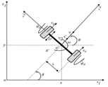
Figure 1 Posture of non-holonomic wheeled mobile robot.

Firstly, we need to define two different coordinate frames:

1. An inertial and global reference frame in the environment, in which the robot moves in. It is denoted as ${\Re }_0\left(O_0,\overrightarrow{i_0},\overrightarrow{j_0},\overrightarrow{k_0}\right)$ :
2. A local frame which is attached to the robot and is denoted as ${\Re }^{\prime }\left(O^{\prime },\overrightarrow{i^{\prime }},\overrightarrow{j^{\prime }},\overrightarrow{k^{\prime }}\right)$ :

The origin of the local robot frame is the mid-point O’ on the axe between the wheels and the centre of mass C is at a distance d from the origin O’.

The posture of any point in the robot can be represented in the local frame as $q^{\prime }={\left(x^{\prime }{y}^{\prime }\theta \right)}^T$ :and in the inertial frame as:$q_I={\left(x_I y_I\theta \right)}^T$

Where:

$x\text{^'},y\text{^'}$ : are coordinates in the local frame,

$x_I, y_I$ : are coordinates in the inertial frame,

$\theta$ : is the angle between the heading direction and the x axis.

The two coordinates are linked by the orthogonal rotation matrix as follows:$R\left(\theta \right)=\left(\begin{array}{ccc}cos\theta & -sin\theta & 0\\ sin\theta & cos\theta & 0\\ 0& 0& 1\end{array}\right)$ (1)

We can apply the same transformation between frames on motions as:${\dot{q}}_I=R\left(\theta \right){\dot{q}}^{\text{'}}$ (2)

This equation is very important, because it defines relations between velocities in the inertial frame and the local frame. In fact, motions of a differential-drive mobile robot are described by two non-holonomic conditions which are:

1. 1^st Condition: in the local robot frame, the velocity of the center-point O’ is zero along the lateral axis:

                                                                                      $\dot{y}=0$ (3)

Considering the orthogonal rotation matrix, the velocity in the inertial frame gives:

                                                                                 $-\dot{x}sin\theta +\dot{y}cos\theta =0$ (4)

II. 2^nd Condition: each wheel maintains one contact point S with the ground. The velocities of the contact points in the robot frame are related to the wheel velocities by:$\{\begin{array}{c}{v}_{sr}=r{\dot{\phi }}_{wr}\\ v_{sl}=r{\dot{\phi }}_{wl}\end{array}$ (5)

${\dot{\phi }}_{wr}and{\dot{\phi }}_{wl}$ Are angular velocities of right and left wheels.

The positions of left and right wheels in the inertial frame are expressed with:

$\{\begin{array}{c}{x}_{wl}=x-Lsin\theta \\ x_{wl}=y+Lcos\theta \end{array} and\{\begin{array}{c}{x}_{wr}=x+Lsin\theta \\ x_{wr}=y-Lcos\theta \end{array}$ (6)

Considering the rotation matrix $R(\theta )$ , the velocities of right and left wheels are given by:

$\{\begin{array}{c}{\dot{x}}_{wl}-r{\dot{\phi }}_{wl}cos\theta =0\\ {\dot{y}}_{wl}-r{\dot{\phi }}_{wl}sin\theta =0\end{array} and \{\begin{array}{c}{\dot{x}}_{wr}-r{\dot{\phi }}_{wr}cos\theta =0\\ {\dot{y}}_{wr}-r{\dot{\phi }}_{wr}sin\theta =0\end{array}$ (7)

Replacing positions equations in the velocities equations, we obtain:

$\{\begin{array}{c}\stackrel{.}{\overbrace{x-L\sin \theta }}-r{\dot{\phi }}_{wl}\cos \theta =0\\ \stackrel{.}{\overbrace{y+Lcos\theta }}-r{\dot{\phi }}_{wl}\sin \theta =0\end{array} and \{\begin{array}{c}\stackrel{.}{\overbrace{x+L\sin \theta }}-r{\dot{\phi }}_{wr}\cos \theta =0\\ \stackrel{.}{\overbrace{y-L\cos \theta }}-r{\dot{\phi }}_{wr}\sin \theta =0\end{array}$ (8)

Thus the rolling constraint equations are formulated as follows:

$\{\begin{array}{c}\begin{array}{c}\dot{x}-L\dot{\theta }cos\theta -r{\dot{\phi }}_{wl}cos\theta =0\\ \dot{y}-L\dot{\theta }sin\theta -r{\dot{\phi }}_{wl}sin\theta =0\end{array}\\ \begin{array}{c}\dot{x}+L\dot{\theta }cos\theta -r{\dot{\phi }}_{wr}cos\theta =0\\ \dot{y}+L\dot{\theta }sin\theta -r{\dot{\phi }}_{wr}sin\theta =0\end{array}\end{array}$ (9)

 We can express these equations by the following matrix$A^T(q$ of non-holonomic constraints:$A^T\left(q\right)=\left(\begin{array}{ccc}-sin\theta & cos\theta & 0\\ cos\theta & sin\theta & L\\ cos\theta & sin\theta & -L\end{array} \begin{array}{c}0\\ -r\\ 0\end{array} \begin{array}{c}0\\ 0\\ -r\end{array}\right)$ (10)

This matrix of constraints and the posture vector verify:

$A^T\left(q\right)\dot{q}=\left(\begin{array}{ccc}-sin\theta & cos\theta & 0\\ cos\theta & sin\theta & L\\ cos\theta & sin\theta & -L\end{array} \begin{array}{c}0\\ -r\\ 0\end{array} \begin{array}{c}0\\ 0\\ -r\end{array}\right)\left(\begin{array}{c}\dot{x}\\ \dot{y}\\ \begin{array}{c}\dot{\theta }\\ {\dot{\phi }}_r\\ {\dot{\phi }}_l\end{array}\end{array}\right)$ (11)

Kinematic model: The main principle of kinematic modeling is to provide relationships between linear and angular robot velocities and angular velocities of left and right wheels. The overall study is based on the mechanical system motion without taking into consideration forces.

From the matrix constraints, we can give the derivative posture as functions of wheels angular velocities:$\{\begin{array}{c}\dot{x}=\frac{r}{2}\left({\dot{\phi }}_{wr}+{\dot{\phi }}_{wl}\right)cos\theta \\ \begin{array}{c}\dot{y}=\frac{r}{2}\left({\dot{\phi }}_{wr}+{\dot{\phi }}_{wl}\right)sin\theta \\ \dot{\theta }=\frac{r}{2L}\left({\dot{\phi }}_{wr}-{\dot{\phi }}_{wl}\right)\end{array}\end{array}$ (12)

The linear velocity of each driving wheel in the robot frame is:

$\{\begin{array}{c}{v}_{wr}=r{\dot{\phi }}_{wr}\\ v_{wl}=r{\dot{\phi }}_{wl}\end{array}$ (13)

Therefore, the linear velocity of the robot is the average of the linear velocities of the two wheels:$v=\frac{1}{2}\left(v_{wr}+v_{wl}\right)=\frac{r}{2}\left({\dot{\phi }}_{wr}+{\dot{\phi }}_{wl}\right)$ (14)

And the angular velocity of the robot is expressed with the two wheels angular velocities as:

(15)

On the contrary, we can obtain the two wheels angular velocities as functions of linear and angular robot velocities as:

${\dot{\phi }}_{wr}=\frac{1}{r}v-\frac{L}{r}\omega and {\dot{\phi }}_{wr}=\frac{1}{r}v+\frac{L}{r}\omega$ (16)

Finally, the forward robot kinematic model is given by:

$\stackrel{.}{q}=\left(\begin{array}{c}\stackrel{.}{x}\\ \stackrel{.}{y}\\ \begin{array}{c}\stackrel{.}{\theta }\\ {\dot{\phi }}_{\text{wr}}\\ {\stackrel{}{\dot{\phi }}}_{\text{wl}}\end{array}\end{array}\right)=\left(\begin{array}{c}\begin{array}{cc}\text{cosθ}& 0\\ \text{sinθ}& 0\\ 0& 1\end{array}\\ \begin{array}{cc}\raisebox{1ex}{$1$}\!\left/ \!\raisebox{-1ex}{$\text{r}$}\right.& -\raisebox{1ex}{$\text{L}$}\!\left/ \!\raisebox{-1ex}{$\text{r}$}\right.\end{array}\\ \begin{array}{cc}\raisebox{1ex}{$1$}\!\left/ \!\raisebox{-1ex}{$\text{r}$}\right.& \raisebox{1ex}{$\text{L}$}\!\left/ \!\raisebox{-1ex}{$\text{r}$}\right.\end{array}\end{array}\right)\left(\begin{array}{c}\text{v}\\ \text{ω}\end{array}\right)$(17)

We can have also this model:

$\dot{q}=\left(\begin{array}{c}\dot{x}\\ \dot{y}\\ \dot{\theta }\\ {\dot{\phi }}_{wr}\\ {\dot{\phi }}_{wl}\end{array}\right)=\left(\begin{array}{cc}r\cos \theta & r\cos \theta \\ r\sin \theta & r\sin \theta \\ \raisebox{1ex}{$r$}\!\left/ \!\raisebox{-1ex}{$2l$}\right.& \raisebox{1ex}{$-r$}\!\left/ \!\raisebox{-1ex}{$2l$}\right.\\ 1& 0\\ 0& 1\end{array}\right)\left(\begin{array}{c}{\dot{\phi }}_{wr}\\ {\dot{\phi }}_{wl}\end{array}\right)$ (18)

Dynamic modelling development

The main purpose is to represent robot dynamic model which is crucial for simulation study of various motion control algorithms design. The robot dynamic model should take into account different forces which affects its motion.

Generally, a non-holonomic differential robot with m constraints, n generalized coordinates and n-m inputs is illustrated by the above motion equation:

$M\left(q\right)\ddot{q}+C\left(q,\dot{q}\right)\dot{q}+F\left(\dot{q}\right)+G\left(q\right)+{\tau }_q=B\left(q\right)\tau +A^T\left(q\right)\lambda$ (19)

where:

$M\left(q\right)\in {\Re }^{n\times m}$ : Is a symmetric positive definite inertia matrix,

$C\left(q,\dot{q}\right) \in {\Re }^{n\times m}$ : Is the centripetal and coriolis matrix,

$F\left(\dot{q}\right)\in {\Re }^{n\times 1}$ : Is the surface friction matrix,

$G\left(q\right)\in {\Re }^{n\times 1}$ : Is the gravitational vector,

${\tau }_p\in R^{\left(n-m\right)*1}$ : Is the bounded unknown disturbance,

$B\left(q\right)\in {\Re }^{n\times \left(n-m\right)}:$ Is the input matrix,

$\tau \in {\Re }^{\left(n-m\right)\times 1}$ Is the control input vector, provided by actuators,

$A^T\left(q\right) :$ Is the matrix associated with the kinematic constraints and verify, and  is the Lagrange multipliers vector.

The approach used for such modeling is the Lagrange dynamic approach.^19,20 The principle of the method is analytically based on the kinetic and potential energies of the system.

The following equation describes the Lagrange equation:$\frac{d}{dt}{\left(\frac{\partial L}{\partial \dot{q}}\right)}^T-{\left(\frac{\partial L}{\partial q}\right)}^T=B\left(q\right)\tau +A^T\left(q\right)\lambda$ (20)

Where:$L(q,\dot{q})=U(q,\dot{q})-T(q)$ (21)

In the Lagrangian function, U is the kinetic energy, T is the potential energy, q is the generalized coordinates, (𝑞) is a matrix that relies actuators torques and generalized forces;

First of all, kinetic and potential energies that govern the motion of the robot should be calculated. And since the robot is moving in the inertial frame, its potential energy is considered to be zero.

The generalized coordinates are selected as:$\dot{q}={\left(\begin{array}{ccc}\dot{x}& \dot{y}& \begin{array}{ccc}\dot{\theta }& {\dot{\phi }}_{\text{w}r}& {\dot{\phi }}_{\text{w}l}\end{array}\end{array}\right)}^T$ (22)

The global kinetic energies of the robot consist on the sum of the kinetic energy of the robot platform with the kinetic energies of the wheels and actuators. This relation is given by:

$U\left(q,\dot{q}\right)=U_c\left(q,\dot{q}\right)+U_{wr}\left(q,\dot{q}\right)+U_{wl}\left(q,\dot{q}\right)$ (23)

Where:

$U_c\left(q,\dot{q}\right)$ is the kinetic energy of the robot platform defined as:$U_c\left(q,\dot{q}\right)=\frac{1}{2}{m}_c{v}_c^2+\frac{1}{2}{I}_c{\dot{\theta }}^2$    (24)

$U_{wr}\left(q,\dot{q}\right) :$ is the kinetic energy of the right wheel given by:

$U_{wr}\left(q,\dot{q}\right)=\frac{1}{2}{m}_w{v}_{wr}^2+\frac{1}{2}{I}_m{\dot{\theta }}^2+\frac{1}{2}{I}_w{\dot{\phi }}_{wr}^2$ (25)

$U_{wl}\left(q,\dot{q}\right)$ Is the kinetic energy of the left wheel given by:

$U_{wl}\left(q,\dot{q}\right)=\frac{1}{2}{m}_w{v}_{wl}^2+\frac{1}{2}{I}_m{\dot{\theta }}^2+\frac{1}{2}{I}_w{\dot{\phi }}_{wl}^2$ (26)

where, m_c is the mass of the robot platform, m_w is the mass of each driving wheel, I_c is the moment of inertia of the robot through the center of mass, I_m is the moment of inertia of each driving wheel with a motor about the wheel axis, and I_w is the moment of inertia of each driving wheel with a motor about the wheel diameter.

With consideration to the center of mass coordinates and the two wheels coordinates in the local frame, these equations depend on the generalized coordinates x and y as:

${\text{U}}_{\text{c}}(\text{q},\stackrel{.}{\text{q}})=\frac{1}{2}{\text{m}}_{\text{c}}({(\stackrel{.}{x}-d\stackrel{.}{\theta \sin \theta })}^2+{(\stackrel{.}{y}+d\stackrel{.}{\theta \cos \theta })}^2)+\frac{1}{2}{\text{I}}_{\text{c}}{\stackrel{.}{\theta }}^2$ (27)

${\text{U}}_{\text{wr}}(\text{q},\stackrel{.}{\text{q}})=\frac{1}{2}{\text{m}}_{\text{w}}({(\stackrel{.}{x}-L\stackrel{.}{\theta }\cos \theta )}^2+{(\stackrel{.}{y}-L\stackrel{.}{\theta }\sin \theta )}^2)+\frac{1}{2}{\text{I}}_{\text{m}}{\stackrel{.}{\theta }}^2+\frac{1}{2}{\text{I}}_{\text{w}}{\dot{\phi }}_{\text{wr}}^2$(28)

${\text{U}}_{\text{wl}}(\text{q},\stackrel{.}{\text{q}})=\frac{1}{2}{\text{m}}_{\text{w}}({(\stackrel{.}{x}+L\stackrel{.}{\theta }\cos \theta )}^2+{(\stackrel{.}{y}+L\stackrel{.}{\theta }\sin \theta )}^2)+\frac{1}{2}{\text{I}}_{\text{m}}{\stackrel{.}{\theta }}^2+\frac{1}{2}{\text{I}}_{\text{w}}{\text{<mi>φ</mi> <mo>˙</mo>}}_{\text{wl}}^2$ (29)

After development and with considering that the Lagrangien is equal to the kinetic energy:

$\text{L}(\text{q},\stackrel{.}{\text{q}})=\text{U}(\text{q},\stackrel{.}{\text{q}})$

The Lagrangien equation is then given by:

$\text{L}(\text{q},\stackrel{.}{\text{q}})=\frac{1}{2}\text{m}({\stackrel{.}{x}}^2+{\stackrel{.}{y}}^2)+{\text{m}}_{\text{c}}\text{d}(\stackrel{.}{y}\cos \theta -\stackrel{.}{x}\sin \theta )\stackrel{.}{\theta }+\frac{1}{2}{\text{I}}_{\text{w}}({\dot{\phi }}_{\text{wr}}^2+{\dot{\phi }}_{\text{wl}}^2)+\frac{1}{2}{\text{Iθ}}^2$ (30)

Where,

$\text{m}={\text{m}}_{\text{c}}+2{\text{m}}_{\text{w}}:$ Is the total mass of the robot,

And $\text{I}={\text{I}}_{\text{c}}+{\text{m}}_{\text{c}}{\text{d}}^2+2{\text{I}}_{\text{m}}+2{\text{m}}_{\text{w}}{\text{L}}^2:$ is the total inertia of the robot.

Applying the Lagrangien derivative equation, different matrixes of the dynamic equation are given by:

$M(q)=\left(\begin{array}{ccccc}m& 0& -m_{c}d\sin \theta & 0& 0\\ 0& m& -m_{c}d\cos \theta & 0& 0\\ -m_{c}d\sin \theta & -m_{c}d\cos \theta & I& 0& 0\\ 0& 0& 0& I_r& 0\\ 0& 0& 0& 0& I_r\end{array}\right)$ (31)

$\text{C}(\text{q},\stackrel{.}{\text{q}})=\left(\begin{array}{c}0\\ 0\\ \begin{array}{c}0\\ 0\\ 0\end{array}\end{array}\begin{array}{c}0\\ 0\\ \begin{array}{c}0\\ 0\\ 0\end{array}\end{array}\begin{array}{c}-{\text{m}}_{\text{c}}\text{dsinθ}\\ -{\text{m}}_{\text{c}}\text{dcosθ}\\ \begin{array}{c}0\\ 0\\ 0\end{array}\end{array}\begin{array}{c}0\\ 0\\ \begin{array}{c}0\\ 0\\ 0\end{array}\end{array}\begin{array}{c}0\\ 0\\ \begin{array}{c}0\\ 0\\ 0\end{array}\end{array}\right)$ (32)

$\text{B}\left(\text{q}\right)=\left(\begin{array}{c}0\\ 0\\ \begin{array}{c}0\\ 1\\ 0\end{array}\end{array}\begin{array}{c}0\\ 0\\ \begin{array}{c}0\\ 0\\ 1\end{array}\end{array}\right)$ (33)

$\text{τ}=\left(\begin{array}{c}{\text{τ}}_{\text{r}}\\ {\text{τ}}_{\text{l}}\end{array}\right)$ (34)

${\text{A}}^{\text{T}}\left(\text{q}\right)\stackrel{.}{\text{q}}=\left(\begin{array}{ccc}-\text{sinθ}& \text{cosθ}& 0\\ \text{cosθ}& \text{sinθ}& \text{L}\\ \text{cosθ}& \text{sinθ}& -\text{L}\end{array}\begin{array}{c}0\\ -\text{r}\\ 0\end{array}\begin{array}{c}0\\ 0\\ -\text{r}\end{array}\right)\left(\begin{array}{c}{\text{λ}}_1\\ {\text{λ}}_2\\ \begin{array}{c}{\text{λ}}_3\\ {\text{λ}}_4\\ {\text{λ}}_5\end{array}\end{array}\right)$(35)

Where:

${\text{τ}}_{\text{r}}{\text{ and τ}}_{\text{l}}$ Are torques control inputs of the robot.

Considering that the Lagrangien coefficients are equal to zero, the robot dynamic model is given by:

$\{\begin{array}{c}(\text{m}+\frac{2{\text{I}}_{\text{w}}}{{\text{r}}^2})\stackrel{.}{v}-{\text{m}}_{\text{c}}d{\text{ω}}^2=\frac{1}{\text{r}}({\text{τ}}_{\text{r}}+{\text{τ}}_{\text{l}})\\ (\frac{2{\text{L}}^2{\text{I}}_{\text{w}}}{{\text{r}}^2}+\text{I})\stackrel{.}{\omega }+{\text{m}}_{\text{c}}d\omega v=\frac{\text{L}}{\text{r}}({\text{τ}}_{\text{r}}-{\text{τ}}_{\text{l}})\end{array}$(36)

Actuators dynamic modelling

In general cases, the driving system of mobile robots is based on an armature-controlled DC motors which are considered as servo actuators. These actuators train the two wheels and drive the mobile robot by providing torques control inputs.

The control inputs of the motors are the armatures voltages E(t) (Figure 2).

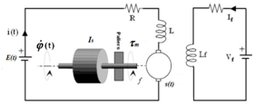
Figure 2 Architecture of a DC motor.

These following equations describe electrical and mechanical parts of the motor circuit:

 $\{\begin{array}{c}E\left(t\right)=Ri\left(t\right)+L\frac{di\left(t\right)}{dt}+e\left(t\right) with e\left(t\right)=K_e{\omega }_m\\ {\tau }_m=I_s\frac{d{\omega }_m\left(t\right)}{dt}+f{\omega }_m\left(t\right)+K_{m}i\left(t\right) with \tau =N{\tau }_m\end{array}$ (37)

Omitting the inertia and the friction of the motor:

$\{\begin{array}{c}\text{E}\left(\text{t}\right)=\text{Ri}\left(\text{t}\right)+\text{L}\frac{\text{di}\left(\text{t}\right)}{\text{dt}}+{\text{K}}_{\text{e}}{\text{ω}}_{\text{m}}\\ {\text{τ}}_{\text{m}}={\text{K}}_{\text{t}}\text{i}\left(\text{t}\right)\text{with τ}={\text{Nτ}}_{\text{m}}\end{array}$ (38)

As motors are mechanically coupled to the wheels by the reducers, mechanical equations of motors are directly linked with those of the robot:

$\{\begin{array}{c}{\text{ω}}_{\text{mr}}=N{\stackrel{.}{\phi }}_{\text{wr }}{\text{and ω}}_{\text{ml}}=N{\stackrel{.}{\phi }}_{\text{wl }}\\ {\text{τ}}_{\text{r}}={\text{Nτ}}_{\text{mr}}{\text{ and τ}}_{\text{l}}={\text{Nτ}}_{\text{ml}}\end{array}$ (39)

Consequently, for the right motor:

$\{\begin{array}{c}{\text{E}}_{\text{r}}\left(\text{p}\right)=(\text{R}+\text{Lp}){\text{i}}_{\text{r}}\left(\text{p}\right)+{\text{K}}_{\text{e}}N{\stackrel{.}{\phi }}_{\text{wr}}\left(\text{p}\right)\\ {\text{τ}}_{\text{mr}}={\text{K}}_{\text{m}}{\text{i}}_{\text{r}}\left(\text{p}\right){\text{with τ}}_{\text{r}}={\text{Nτ}}_{\text{mr}}\end{array}$ (40)

And for the left motor:

$\{\begin{array}{c}{\text{E}}_{\text{l}}\left(\text{p}\right)=(\text{R}+\text{Lp}){\text{i}}_{\text{l}}\left(\text{p}\right)+{\text{K}}_{\text{e}}N{\stackrel{.}{\phi }}_{\text{wl}}\left(\text{p}\right)\\ {\text{τ}}_{\text{ml}}={\text{K}}_{\text{m}}{\text{i}}_{\text{l}}\left(\text{p}\right){\text{with τ}}_{\text{l}}={\text{Nτ}}_{\text{ml}}\end{array}$ (41)

As a result, the obtained equations are the dynamic model of the two motors:

$\{\begin{array}{c}\begin{array}{c}\frac{1}{(\text{R}+\text{Lp})}({\text{E}}_{\text{r}}-{\text{K}}_{\text{e}}N{\stackrel{.}{\phi }}_{\text{wr}})={\text{i}}_{\text{r}}{\text{ and τ}}_{\text{r}}={\text{Nτ}}_{\text{mr}}\\ \frac{1}{(\text{R}+\text{Lp})}({\text{E}}_{\text{l}}-{\text{K}}_{\text{e}}N{\stackrel{.}{\phi }}_{\text{wl}})={\text{i}}_{\text{l}}{\text{ and τ}}_{\text{l}}={\text{Nτ}}_{\text{ml}}\end{array}\\ \end{array}$ (42)

The dynamic equations of the mobile robot and those of the actuators are given by this scheme: (Figure 3)

The closed loop feedback scheme in which angular velocities references of the right and the left wheels are considered as inputs, is given by the Figure 4.

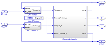
Figure 3 Open loop dynamical robot system developed on SIMULINK software.

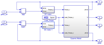
Figure 4 Closed loop scheme of dynamical robot system developed on SIMULINK software.

Different control strategies are used and designed for both speed control of DC motors and trajectory tracking for mobile robots.

In this section, the trajectory tracking and the speed control problems for the mobile robot are presented even in the presence of load torques T_lr and T_ll which are applied to test the system’s control performances. This applied load torques T_lr and T_ll are used to model the obstacles in the form of holes and the stones in the hostile environment in which the robot is evolving. The problematic is that the robot moves in a hostile environment full of holes and stones and must behave in an autonomous manner. The control objective is to design a controller which can adapt the mobile robot behavior to the application of different load torques. 

In fact, it is important to know that the couple: load torque and robot behavior must be correspondent and must respect some rules:

1. If ${\text{T}}_{\text{lr}}\left({\text{respectively T}}_{\text{ll}}\right)<{\text{τ}}_{\text{r}}\left({\text{respectively τ}}_{\text{l}}\right)$ that is the load torques are less than the robot wheels torques, so the robot can overcome the obstacles (soft holes or stones), and then should evolve normally in its trajectory without changing its behaviour;
2. If ${\text{T}}_{\text{lr}}\left({\text{respectively T}}_{\text{ll}}\right)>{\text{τ}}_{\text{r}}\left({\text{respectively τ}}_{\text{l}}\right)$ that is the load torques are higher than the robot wheels torques, thus the robot should try to overcome the obstacles ( medium holes or stones), brake and then continue its trajectory normally ;
3. If ${\text{T}}_{\text{lr}}\left({\text{respectively T}}_{\text{ll}}\right)>>{\text{τ}}_{\text{r}}\left({\text{respectively τ}}_{\text{l}}\right)$ that is the load torques are extremely higher than the robot wheels torques, hence the obstacles are quite difficult to overcome (very deep holes or big stones), then the robot should STOP to avoid motors damages, bypass and encounter the obstacles ;
4. If $T_{Ir}>T_{Il}$ that is the left load torque is less than the right load torque ( left obstacle is less important than the right one), then the robot should turn to the LEFT;
5. If ${\text{T}}_{\text{lr}}<{\text{T}}_{\text{ll}}$ that is the left load torque is higher than the right load torque (left obstacle is more important than the right one), then the robot should turn to the RIGHT.

Our case study is based on two controller strategies: a classical PID controller (CPIDC) and a Real Time Dynamic PID optimized Neural Networks Controller (RTDPID). These two controllers were implemented on Matlab/Simulink environment and a comparative study is presented to demonstrate the effectiveness of the proposed smart control strategy based on neural networks.

Classical PID controller (CPIDC)

PID controller is a standard control feedback loop method commonly used in industry. The essential mission of PID controllers consists in reducing to zero the error between output or measured process variable and a desired set point by calculating and then outputting a corrective action that can adjust the process accordingly.

Since PID controllers are well recognized for achieving desired behavior, the control design should attend the goals which are: speed control and trajectory tracking even with the presence of load torques T_lr and T_ll and without affecting the overall system stability.

In this section, a closed loop feedback algorithm based on PID controller has been developed for precise position, speed control, and especially for testing the behaviour of mobile robot regarding load torque application.

PID structure consists of proportional, integral and derivative actions which are implemented in parallel form. The derivative term is used to reduce the overshoot by improving the transient response and stabilizing the overall system behaviour, and the Integral term is used to reduce steady state error in a control system.

This classical PID controller is represented with its well known continuous transfer function as follows:

$C\left(p\right)=K_p+\frac{K_I}{p}+K_{D}p$ (43)

Where k_P, k_I and k_D refer to proportional, integral and derivative gain constants respectively.

The tuning of these coefficients is done based on the Ziegler and Nichols approach considering the closed loop scheme. The main advantage of this method is its simplicity, and it consists in setting the integral K_I gain to the maximum, and derivative K_D gain to zero.

However, the proportional K_P gain is then increased until it reaches the critical gain K_osc, and the system oscillates continuously among constant amplitude oscillations with T_osc period. Then K_osc and T_osc are used to set the PID gains based on mathematical approximations.²¹

The simulation leads to: (Figure 5)

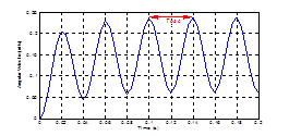
Figure 5 Response of Ziegler and Nichols approach.

Where: T_osc=0.04s with K_osc=15.

By tuning these three constants, the PID controller algorithm can provide control action designed to let velocities of the wheels and the robot following desired specific process requirements, and mainly to test the behaviour of mobile robot against load torque application.

The closed loop PID control scheme is represented as: Figure 6

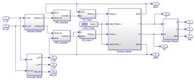
Figure 6 Closed loop PID control scheme.

The inputs of the closed loop system are references of linear and angular velocities of the robot $\text{V}\_\text{ref and W}\_\text{ref}$ , and the outputs are linear and angular velocities of the robot $\text{V and W}$ , angular velocities of the wheels ${\dot{\phi }}_{wr} and {\dot{\phi }}_{wl}$ , x, y positions and the angle $\theta$ .

Real time dynamic PID optimized neural networks controller (RTDPID)

In this section, the main idea is to optimize PID controller coefficients with the use of neural networks method.

Neural network architecture: The neural network utilised is a multi-layer network with the most popular training method, which is the back-propagation algorithm. Its structure is composed of three layers: the first one is the intput layer, the second is the hidden layer and the third is the output layer.

The first layer is constituted of four inputs which are the two errors between angular velocities of the wheels ${\stackrel{.}{\phi }}_{\text{wr }}and{\stackrel{.}{\phi }}_{\text{wl }}$ and their referencesand the two armature voltages of the two motors, the second layer is composed of eighteen hidden neurons with “tansigmoid” activation functions and the third layer have three outputs “purelin” neuron which are the coefficients of the PID controller k_P, k_I and k_D. So, for this application, the neural network is expected to provide the optimal PID coefficients for the mobile robot control behaviour against some load torques.

Learning phase: The back-propagation algorithm trains the neural network. In a typical back-propagation training session, the supervisor presents input data to the network and compares the network’s actual output O_p to the target (or desired) output T_p. The basis of this comparison is the adjustment of weights w_ij and biases b_ij in order to reduce the value of a certain criterion: the energy function E represented by this equation:

$\text{E}=\frac{1}{2}{\left({\text{T}}_{\text{p}}-{\text{O}}_{\text{p}}\right)}^2$ (44)

This difference is used to change the connection weights between neurons in the network as:

${\text{Δω}}_{\text{j}}\left(\text{t}+1\right)=\text{η}\left(-\frac{\partial \text{E}}{\partial {\text{ω}}_{\text{j}}}\right)+{\text{αΔω}}_{\text{j}}\left(\text{t}\right)$ (45)

By this way, the weights are adjusted in a gradient descent manner, which means the minimization of the error between the expected output and the actual output for a particular input.

For training purpose and tests, some data sets were created from the closed loop feedback scheme describing the mobile robot desired behavior against load torque application.

Closed loop real time dynamic PID optimized neural networks controller: Figure 7 shows the proposed strategy of mobile robot control. It is a task of replacing both classical PID controllers with one Real Time Dynamic PID optimized Neural Networks Controller. This neural network is asked to learn information about a data set, in order to compute a number of weights that best allow the controller to track the given input/output data, in order to provide PID controller with the optimal values of its coefficients {k_P, k_I, k_D} corresponding to the desired mobile robot behavior.

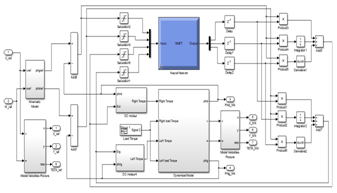
Figure 7 PID optimized Neural Networks controller scheme.

Once the interconnection weights and the biaises are adjusted according to the desired output, these neural models are incorporated in the control loop of the overall controlled system, and are used as one controller providing the inverter with the appropriate voltage vector.

The neural networks utilised are the same as the one described in the previous section. However, its structure is quite different.

The training design of the PID and the neural optimized PID controllers are achieved with the environment of Matlab/Simulink and a comparative study is carried out in a hostile environment with respect to various disturbances that can be holes and stones modeled by different load torques. The controlled robot must be autonomous for the decision making: it can decelerate and then continue its trajectory or stop depending on the size of the obstacles, thus avoiding the damage of the engine, or change its trajectory if needed.

The table below resumes the applied load torques and the desired behavior of the mobile robot with considering that the motor torque maximum is 25N.m (Table 1).

The control strategy, as follows, consists of applying:

1. A linear velocity reference $\text{V}\_\text{ref}=1m/s$ ;
2. An angular velocity reference $W\_ref=0.5rd/s$ ;
3. A load torque reference as follows: (Figure 8)

The following figures represent results of both training control lows with different cases studies.

Figure 8 Load Torque Reference.

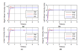
1st case study: Load torque<Motor torque: (20 N.m)

Figure 9 Simulation results of PID and NN Controllers: (a-b) Right and Left Wheels Velocities, (c-d) Linear and Angular Velocities.

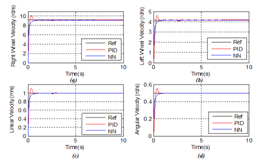
2nd case study: Load torque>Motor torque: (35 N.m)

Figure 10 Simulation results of PID and NN Controllers: (a-b) Right and Left Wheels Velocities, (c-d) Linear and Angular Velocities.

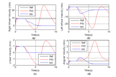
3rd case study: Load torque>>Motor torque (53 N.m)

Figure 11 Simulation results of PID and NN Controllers: (a-b) Right and Left Wheels Velocities, (c-d) Linear and Angular Velocities.

Figure 12 Circular Trajectories: (a) PID Controller, (b) NN Controller

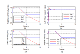
4th case study: Right Load torque > Left Load torque $T_{lr}\left(52 Nm\right)>T_{ll}\left(45 Nm\right)$

(c-d) Linear and Angular Velocities.

Figure 13 Simulation results of PID and NN Controllers: (a-b) Right and Left Wheels Velocities, (c-d) Linear and Angular Velocities.

5th case study: Right Load torque < Left Load torque${\text{T}}_{\text{lr}}\left(30\text{ Nm}\right)<{\text{T}}_{\text{ll}}\left(50\text{ Nm}\right)$

Figure 14 Simulation results of PID and NN Controllers: (a-b) Right and Left Wheels Velocities, (c-d) Linear and Angular Velocities.

In the previous section, four cases of desired behaviors were applied to our smart robot and the velocities responses were exposed taking into account the application of different load torques and the effects that they have on these responses. In all of the figures we have considered the responses of both right and left wheels velocities and both of linear and angular velocities. In fact, “Figure 9” represents the case of a load torque equal to 20 N.m that is less than the motors torques, we notice that the robot continue normally its navigation and he wasn’t affected by the load torque presence. In the second case, we have applied a load torque of 35 N.m that is higher than the motors torques we have noticed by “Fig.10” that speed responses evolves with low variations at the time of load torque application followed by speed compensation, in addition the static error is equal to zero which makes the system quite accurate. “Figure 11” presents the case of a load torque equal to 53 N.m which is much more important than the motors torques; we remark that behavior satisfy the specifications imposed in the table below and is able to achieve the goal. In fact, the robot stops for fear to damage the motors wheels that are training the robot. In the contrary, PID controllers allow bad responses in the way that the overall system became instable. Moreover, “Figure12” shows that the controlled PID robot is not able to follow circular trajectory that is the system is instable.  “Figure13” and “Figure14” presents two cases studies of applying different load torques on the left and right wheels; we noticed that the RTDPID optimized Neural Networks Controller permit better behavior. In fact, when applying a right wheel load torque superior to the left wheel load torque, the right wheel decelerate and the left wheel accelerate which forces the robot to turn to the right and vice versa. Basically, the RTDPID optimized Neural Networks Controller allows improved responses of the velocities while varying the intensities of obstacles by applying some load torques with different degrees. In fact, in the case of RTDPID optimized Neural Networks Controller, the robot can be qualified as a smart robot evolving in a hostile environment and this control strategy can be considered as a robust technique that obeys the desired and imposed specifications resumed in the table below. By the way, it might also be noted that the robot is smart, intelligent and answers quickly while keeping the system stable. In addition, the robot conserves its circular trajectory in the first and second control cases except the third case study in which the robot loses its stability. In the previous section, four cases of desired behaviors were applied to our smart robot and the velocities responses were exposed taking into account the application of different load torques and the effects that they have on these responses. In all of the figures we have considered the responses of both right and left wheels velocities and both of linear and angular velocities. In fact, “Figure 9” represents the case of a load torque equal to 20 N.m that is less than the motors torques, we notice that the robot continues its navigation normally and it is not affected by the load torque presence. In the second case, we have applied a load torque of 35 N.m that is higher than the motors torques we have noticed by “Figure 10” that speed responses evolves with low variations at the time of load torque application followed by speed compensation. In addition, the static error is equal to zero which makes the system quite accurate.

“Figure 11” presents the case of a load torque equal to 53 N.m which is much more important than the motors torques; we remark that behavior satisfy the specifications imposed in the table below and is able to achieve the goal. In fact, the robot stops for fear it damages the motors wheels that are training the robot. On the contrary, PID controllers allow bad responses and as a result the overall system became instable. Moreover, “Figure 12” shows that the controlled PID robot is not able to follow circular trajectory meaning that the system is instable.  “Figure13” and “Figure 14” present two case studies of applying different load torques on the left and right wheels, we noticed that the RTDPID optimized Neural Networks Controller permit better behavior. In fact, when applying a right wheel load torque superior to the left wheel load torque, the right wheel decelerates and the left wheel accelerates which forces the robot to turn to the right and vice versa.  Basically, the RTDPID optimized Neural Networks Controller allows improved responses of the velocities while varying the intensities of obstacles by applying some load torques with different degrees. In fact, in the case of RTDPID optimized Neural Networks Controller, the robot can be qualified as a smart robot evolving in a hostile environment and this control strategy can be considered as a robust technique that obeys the desired and imposed specifications resumed in the table below. It might also be noted that the robot is smart, intelligent and answers quickly while keeping the system stable. In addition, the robot conserves its circular trajectory in the first and second control cases except the third case study in which the robot loses its stability (Figure 15).

Figure 15 Circular Trajectories: (a) PID Controller, (b) NN Controller.

In this paper, an RTDPID optimized Neural Networks Control scheme was proposed for a two-wheeled non-holonomic robot progressing in a hostile environment. It was shown that the controller is robust against different and intensive load torques and also guarantees stability and precision for static error performances. This control scheme resolves the problem of actuators damages when the robot meets undesirable obstacles. Simulation results of the mobile robot model were given to ensure the effectiveness of the controlled system.

Moreover, the RTDPID optimized neural network control technique gives better results when compared with the classical PID controller. This success is revealed by the behavior of the robot when tracking trajectories, avoiding obstacles and assuring both stability and accuracy.

Eventually, we can be assured that we have extended the aim of this work. In fact, when evolving in a hostile environment, the controlled robot is autonomous in decision making: it decelerates and then continues its trajectory, stops depending on the size of the obstacles, and as a result avoids damage to the motors, or turns to the left or to the right. It is also smart and able to protect itself against high load torques without affecting, neither its trajectory tracking nor its stability. In this context, the future scope of such smart robot is relatively very high. There are various applications which can be easily applied using other tools and technologies. The most important tool that can be considered is the use of deep learning instead of neural networks that are trainable “brains”. In fact, as robots are designed for a range of behaviors in a plethora of environments, Self-supervised learning approaches enable robots to generate their own training examples in order to improve performances. As future scope to our work, we can apply the self-supervised learning method to road and objects detection, identification of obstacles in rough terrain and in a 3D-scene analysis and modeling.

None.

None.

The author declares there are no conflicts of interest.

1. Yang H, Xiaozhao Fan, Peng Shi, et al. Nonlinear Control for Tracking and Obstacle Avoidance of a Wheeled Mobile Robot With Nonholonomic Constraint. IEEE Transactions on Control Systems Technology. 2016;24(2):741–746.
2. Julio ENR, Ismael A, Juan GO, et al. Mobile robot path tracking using a robust PID controller. Control Engineering Practice. 2001;9(11):1209–1214.
3. Ye J. Adaptive control of nonlinear PID-based analog neural networks for a nonholonomic mobile robot. Neurocomputing. 2008;71(7–9):1561–1565.
4. Roy S,Nandy S, Ray R, et al. Robust Path Tracking Control of Nonholonomic Wheeled Mobile Robot: Experimental Validation. International Journal of Control, Automation and Systems. 2015;13(4):897–905.
5. Kazuya S, Masahiro Y, Kazuhiro T. Robust Adaptive Trajectory Control of Nonholonomic Mobile Robot with Compensation of Input Uncertainty. Journal of System Design and Dynamics. 2012;6(3):273–286.
6. Koubaa Y, Boukattaya M, Dammak T. Adaptive Sliding–Mode Dynamic Control For Path Tracking of Nonholonomic Wheeled Mobile Robot. J. Automation & Systems Engineering. 2015;9(2):119–131.
7. Yang J, Ma R, Zhang Y, et al. Sliding Mode Control for Trajectory Tracking of Intelligent Vehicle. Physics Procedia. 2012;33:1160–1167.
8. Rossomando FG, Soria C, Carelli R. Sliding Mode Neuro Adaptive Control in Trajectory Tracking for Mobile Robots. Journal of Intelligent & Robotic Systems. 2014;74(3–4):931–944.
9. Park BS, Yoo SJ, Park JB, et al. A Simple Adaptive Control Approach for Trajectory Tracking of Electrically Driven Nonholonomic Mobile Robots. IEEE Transactions on Control System Technology. 2010;18(5):1199–1206.
10. Fukao T, Nakagawa H, Adachi N. Adaptive tracking control of a nonholonomic mobile robot. IEEE Transactions on Robotics and Automation. 2000;16(5):609–615.
11. Das T, Kar IN. Design and implementation of an adaptive fuzzy logic-based controller for wheeled mobile robots. IEEE Transactions on Control System Technology. 2006;14(3):501–510.
12. Abadi DNM, Khooban MH. Design of optimal Mamdani-type fuzzy controller for nonholonomic wheeled mobile robots. Journal of King Saud University-Engineering Science. 2015;27(1):92–100.
13. Abdessemed F, Benmahammed KH, Monacelli E. A fuzzy based reactive controller for a non-holonomic mobile robot. Robotics And Autonomous Systems. 2004;47(1):31–46.
14. Khnissi K, Seddik C, Seddik H. Smart Navigation of Mobile Robot Using Neural Network Controller. 2018 International Conference onSmart Communications in Network Technologies (SaCoNet); 2018 october 27–31: Nigeria: IEEE; 2018.
15. Ye J. Tracking control of a non-holonomic wheeled mobile robot using improved compound cosine function neural networks. International Journal of Control. 2014;88(2):364–373.
16. Michel LF, Edgar NS, Alma YA, et al. Neural Control for a Differential Drive Wheeled Mobile Robot Integrating Stereo Vision Feedback.  Computacion y Sistemas. 2015;19(3):429–443.
17. Salem FA. Dynamic and Kinematic Models and Control for Differential Drive Mobile Robots. International Journal of Current Engineering and Technology. 2013;3(2):253–256.
18. Cerkala J, Jadlovska A. Nonholonomic mobile robot with differential chassis mathematical modelling and implementation in simulink with friction in Dynamics. Acta Electrotechnica et Informatica. 2015;15(3):3–8.
19. Ito K, Kunisch K. Lagrange Multiplier Approach to Variational Problems and Applications. Advances in Design and Control. 2008.
20. Dhaouadi R, Abu Hatab A. Dynamic Modelling of Differential-Drive Mobile Robots using Lagrange and Newton-Euler Methodologies: A Unified Framework. Advances in Robot and Automation. 2013;2(20):1–7.
21. Astrom KJ, Hagglund T. Revisiting the Ziegler–Nichols step response method for PID control. Journal of Process Control. 2004;14:635–650.