The conventional PID controller is very good when all parameters of the system are Known, that’s mean the system is linear, but when the system is nonlinear because of the friction, the saturation, the disturbance, or the load the dynamic model of the system will be the change, in this case, the conventional PID controller is not good, therefore we used the FLC because it is considered as intelligent controller and it is very suitable when parameter changed or not known, FLC does not need to now the all dynamic model of the system, that’s mean FLC is good with nonlinear system. In this paper, we presented the modeling of DC Motor, and how to compute the full dynamic model of DC Motor, after that we built a subsystem for DC Motor using MATLAB / Simulink, then we applied the PID controller and fuzzy logic controller for controlling the speed of DC Motor, the parameters of PID controller proportional (P), integral (I), derivative (D), tuned by using PID tuning tool in Simulink, we designed FLC for speed control, then we compared the simulation results between PID and FLC, in characteristics rise time, settling time, steady-state error and overshoot. From the simulation results and table compared we found that the performance of FLC is better than the performance of the PID controller in terms of speed control in case of no disturbance or load and with disturbance or load.

Keywords: Fuzzy logic controller (FLC), PID controller, DC motor, speed controls

Direct Current (DC) motor is one of the widest actuators utilized in various control applications including driven an automated controller, tape transport systems, circle drives, machine apparatuses, and servo valve actuators, that is because a DC motor has highlights, for example, high force, speed controllability over a wide reach, less expensive and calmer, compactness, polite speed-force qualities, flexibility to different sorts of control techniques.

To control the dc motor we used PID controller and FLC, the practical problem that we study in this work is implementing PID controller, it is not suitable with the nonlinear system because of the friction, the actuator saturation, the integral windup, and the load or disturbance.

Many papers study this problem, for example, papers^1–11 these papers study control in DC Motor with PID controller and fuzzy logic controller, the conclusions from these papers were that performance of fuzzy logic controller was better than the performance of PID controller.

The DC motor needs modeling before applying the control system on it, this modeling refers to the plant system in the mathematical model, which characterizes a transfer function contained on the input and output variables.^12,13

The extraction of a DC motor as a linear device would be the input voltage applied to the field or armature, as well as second-order effects like hysteresis and voltage drop through the brushes, making this a near-equivalent to a real motor, being ignored., another name of DC motor is an actuator that is used to move loads, and it is about a device which provides the driving energy to a load.¹⁴ Figure 1 below shows the electric circuit and mechanical model of a DC motor.

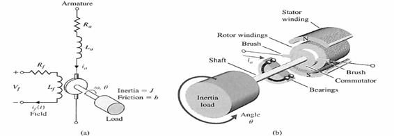
Figure 1 The DC Motor. (a) Wiring diagram. (b) Sketch.

The rotor (armature) of the motor generated the fraction of the torque for driving an external load.¹⁸

As a result, the air gap and the current field are proportional

$\varnothing =Kfif$   (1)

Where

The magnetic flux is $\varnothing$ , a proportional constant is $kf$  and The field current is $if$ .

The armature current and the torque produced by the motor are presumed to be linear to $\varnothing$ related as follows:

$Tm=K1\varnothing ia\left(t\right)=K1Kfif\left(t\right)ia\left(t\right)$ .  (2)

Where

$Tm$  The motor torque. $K1$  a proportional constant. $ia\left(t\right)$  the armature current in (t) domain.

We can deduct from (2) to obtain a linear variable, each current will be kept constant while one becomes the input current.

With Field

The DC motor-operated current field for producing big power execution is the first thing we'll look at. We'll use the Laplace transform notation after that.

$Tm\left(s\right)=\left(K1KfIa\right)If\left(s\right)=KmIf\left(s\right)$ ,  (3)

Where $ia=Ia$  means the current of the armature is constant and $km$  is the Motor constant, variable (S) refers to the S- domain. Figure 2 shows the related voltage and current field.

$Vf\left(s\right)=\left(Rf+Lfs\right)If\left(s\right)$   (4)

Figure 2 Schematic diagram of DC motor field controlled.

$Tm\left(s\right)$  is the motor torque that delivered torque to the load.

$Tm\left(s\right)=TL\left(s\right)+Td\left(s\right)$ ,  (5)

The disturbance torque is $Td(s)$ , and the load torque is $TL(s)$ . For the models exposed to the external power, the disturbance torque must frequently be considered.¹⁴

 Figure 1 shows the load torque for rotating inertia, which we can write as

$TL(s)=J{s}^2\theta (s)+bs\theta (s)$   (6)

From the equations (3), (4), and (5), are combined we obtain

$TL\left(s\right)=Tm\left(s\right)-Td\left(s\right)$ ,  (7)

$Tm\left(s\right)=KmIf\left(s\right)$ ,  (8)

$If\left(s\right)=\frac{Vf\left(s\right)}{Rf+Lfs}$   (9)

The load of the motor, with $Td\left(s\right)=0$ , is

$G\left(s\right)=\frac{\theta \left(s\right)}{Vf\left(s\right)}=\frac{Km}{s\left(Js+b\right)\left(Lfs+Rf\right)} =\frac{Km/\left(JLf\right)}{s\left(s+b/J\right)\left(s+Rf/Lf\right)}$   (10)

Figure 3 shows a DC motor powered by a field. Another alternative is to write the variables in the time constant of the DC motor as a transfer function:

$\frac{\theta \left(s\right)}{Vf\left(s\right)}=G\left(s\right)=\frac{Km/\left(bRf\right)}{s\left(\tau fs+1\right)\left(\tau Ls+1\right)}$ ,  (11)

Figure 3 The DC Motor model controlled by field.

Where $\tau f=Lf/Rf$  and $\tau L=J/b$ . Usually, we find that $\tau L>\tau f$  and often the field time constant is often ignored.¹⁴

With armature

In the armature-controlled DC motor, the armature current ia was used as a control variable. A field coil, current, or a constant generator may be used to construct the stator field.¹⁴ As depicted in Figure 4.

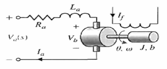
Figure 4 DC motor armature controlled.

When a steady field current is produced in a field coil, the motor torque is increased.

$Tm\left(s\right)=\left(K1KfIf\right)Ia\left(s\right)=KmIa\left(s\right)$ .  (12)

When we use a permanent magnet, we get

$Tm\left(s\right)=KmIa\left(s\right)$ ,  (13)

Where $Km$  is the magnetic permeability feature.

The armature current and input voltage is connected by

$Va\left(s\right)=\left(Ra+Las\right)Ia\left(s\right)+Vb\left(s\right)$ ,  (14)

 The voltage back magnetic field proportional to the motor speed is denoted by $Vb\left(s\right)$ .

$Vb\left(s\right)=Kbw\left(s\right)$ ,  (15)

Where $w\left(s\right)=s\theta \left(s\right)$  is the angular velocity transformation and the armature current is

$Ia\left(s\right)=\frac{Va\left(s\right)-Kbw\left(s\right)}{Ra+Las}$   (16)

The load torque represent by (6) and (7), for

$TL\left(s\right)=J{s}^2\theta \left(s\right)+bs\theta \left(s\right)=Tm\left(s\right)-Td\left(s\right)$ .  (17)

The model in Figure 5 shows a DC motor controlled by armature as a block diagram. We solve for the transfer function using (12), (16), and (17) or the block diagram, thus ignoring disturbance torque $Td\left(s\right)=0$ .

$G\left(s\right)=\frac{\theta \left(s\right)}{Va\left(s\right)}=\frac{Km}{s\left[\left(Ra+Las\right)\left(Js+b\right)+KbKm\right]} =\frac{Km}{s\left(s^2+2\zeta wns+w{n}^2\right)}$   (18)

Figure 5 The DC Motor model is controlled by the armature.

 Fortunately, the armature's time constant, $\tau a=La/Ra$ , is negligible in many DC Motors, so

$G\left(s\right)=\frac{\theta \left(s\right)}{Va\left(s\right)}=\frac{Km}{s\left[Ra\left(Js+b\right)+KbKm\right]}= \frac{Km/\left(Rab+KbKm\right)}{s\left(\tau 1s+1\right)}$ ,  (19)

Where the equivalent time constant $\tau 1=RaJ/\left(Rab+KbKm\right)$ .

It's worth remembering that $Km$  is the same as $Kb$ . When considering the process of engine stability and energy balance while ignoring rotor resistance, this equality can appear. The rotor's power input is $\left(kbw\right)ia$ , and the shaft's power delivery is $Tw$ . The power input is equal to the power supplied to the shaft in the steady-state situation, so $\left(kbw\right)ia=Tw$ , because $T=Kmia$ from (12), we find that $Kb=Km$ . Where a quick response is not needed and only a small amount of power is required, electric motors are used to transfer load.¹⁴

DC motor limits

DC-Motors are torque and speed limited; the maximum current provided by the drive electronics controls maximum torque; a DC-Motor also has a maximum rated current; after this rated current, a DC-Motor may be affected by overheating or de-magnetization; as a result, a permanent magnet that decreases its torque constant permanently is used. Any increase in speed decreases friction, and the maximum speed is defined as follows:

$w_{max}={\tau }_{max}/B$ , where w is speed, τ is torque and B is friction, the product of motor torque and speed is the mechanical output power.¹²

In the Table 1 below we used these values for the parameters of the DC motor simulation.

PID Controller

The PID controller is the abbreviation for the Proportional Integral Derivative controller it is considered as a controller of feedback, although it is a conventional controller, it is still widely used in the industry. The idea of controlling the work is simple, and it is to calculate the difference between the actual income of the system and the output.^15–17

The proportional part plus integral part plus derivative part is called control action and defined by:

$u\left(t\right)=Kpe\left(t\right)+\frac{Kp}{Ti}{{\displaystyle \int }}_0^{t}e\left(t\right)d\left(t\right)+KpTd\frac{de\left(t\right)}{d\left(t\right)}$   (20)

$Gc\left(s\right)=\frac{U\left(s\right)}{E\left(s\right)}=Kp\left(1+\frac{1}{Tis}+Tds\right)$   (21)

This controller is used to improve both transient and steady-state responses. It has advantages over the three individual control actions, Figure 6 shows the PID Controller in a close loop system.

Figure 6 The PID-controller.

Where $E\left(s\right)=R\left(s\right)-Y\left(s\right)$  

Which represents the input value minus the output value. The proportional control $\left(Kp\right)$  reduces the rise time and the steady-state error but does not eliminate it. The integral control $\left(Ki\right)$ eliminates the steady-state error, but it may affect the transient response and make it worse. The stability and transient response improve by derivative control $\left(Kd\right)$  and the overshoot is reduced.

Tuning methods

Tune means a choose numerical values for the PID coefficients and there are many methods for tuning a PID Controller, and then obtaining the desired response, some of these methods are:

1- Ziegler Nichols Methods.

2- The Cohen-Coon Method.

3- The Chien, Hrones and Reswick Method.

4- Trial and Error Method.

5- Manual Tuning Method.

6- Software Method.

In this simulation we used the software method, as follows:

In this method, we used Toolbox inside Simulink in MATLAB called PID Tuning, by this tool we can automatically tune PID controller gains, and find the value of a proportional (P), integral (I), and derivative (D) gains to achieve desired performance.

Integral windup and actuator saturation

One of the practical problems of implementing a PID controller is actuator saturation and integral windup since the range of movement in say a control value has a physical limit once it has saturated increasing the magnitude of the control signal further has little effect.

When the error term varies and the expected and measured values differ, the resulting error causes integral windup, which is a constant rise in the integral term. When an integral term is signed, it starts to unwind, possibly creating long delays and uncertainty. The solution is to limit the maximum value of the integral expression.

Fuzzy logic controller

The following steps demonstrate how to construct a fuzzy logic controller

Define FLC's inputs and outputs. FLC has two inputs: error and error change, as well as one output that is a control signal to the plant.^15,16

1- We chose two inputs with seven membership functions and one output with seven membership functions for the design.

2- The membership role was changed from a negative big NB to a positive big PB in the design.

3- Choose the inference mechanism rule, in this work we chose the Mamdani.

4- The defuzzification approach was used in this work was the center of gravity (COG) (Figure 7–9) (Table 2).

Figure 7 Error.

Figure 8 Change of error.

Figure 9 Output.
NB stands for Negative Big, NM for Negative Medium, NS for Negative Small, ZE for Zero, PS for Positive Small, PM for Positive Medium, and PB for Positive Big.

In this model in Figure 10 below we built the DC Motor model in a subsystem with 2 inputs 2 outputs, the 2 inputs were armature voltage (Va) and disturbance torque (Td), the 2 outputs was angular speed (W) and position (theta), the values for the various parameters taken from Table 1.

Figure 10 The DC motor model in subsystem.

Simulation DC motor using PID controller

Without disturbance

The Simulink model of DC motor with PID controller is shown in Figure 11 below.

Figure 11 Block diagram of DC motor with PID controller.

We simulate the DC Motor with PID controller, in this simulate we applied step input to a PID controller, the speed time response of the DC motor is shown in Figure 12, where the Brown line refers to the desired signal, the Blue line refers to a simulation result.

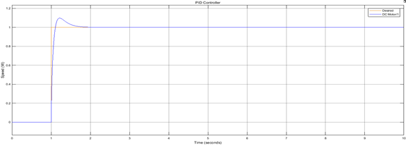
Figure 12 Position response of DC motor using PID controller.

With disturbance

The Simulink model of DC motor with PID controller with 0.05 disturbance is shown in Figure 13 below.

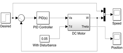
Figure 13 Block Diagram of DC Motor with PID Controller with disturbance.

We simulate the DC Motor with a PID controller with disturbance, in this simulate we applied step input to a PID controller, and 0.05 disturbance Figure 14 shows the simulation result of the DC motor.

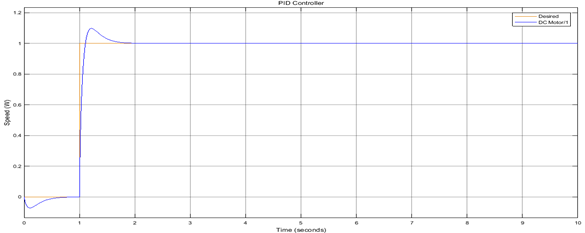
Figure 14 Simulation result of DC Motor Using PID Controller with disturbance.

Simulation DC motor using fuzzy logic controller

Without disturbance

Simulink model of DC motor controlled by Fuzzy Logic is shown in Figure 15 below.

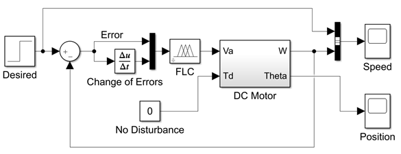
Figure 15 Simulink model of DC Motor controlled by Fuzzy logic.

We simulate the DC Motor with Fuzzy Logic Controller, in this simulate we applied step input to the Fuzzy Logic Controller, Figure 16 shows the speed time response of the DC motor, where the Brown line refers to the desired signal, the Blue line refers to a simulation of FLC result.

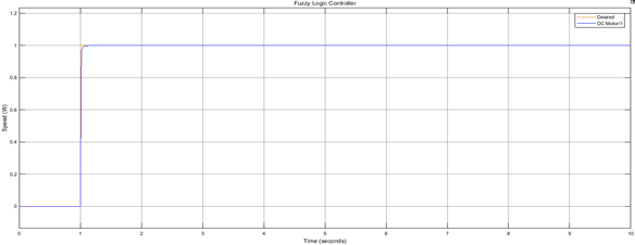
Figure 16 Simulation result of DC Motor Using Fuzzy Logic Controller.

With disturbance

Simulink model of DC motor controlled by Fuzzy Logic with 0.05 disturbance is shown in Figure 17 below.

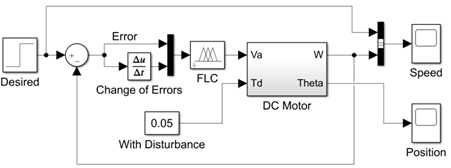
Figure 17 Simulink model of DC Motor controlled by fuzzy logic with disturbance.

We simulate the DC Motor with a Fuzzy Logic Controller, in this simulate we applied step input to the Fuzzy Logic Controller, with 0.05 disturbance Figure 18 shows the speed time response of the DC motor (Table 3 & 4).

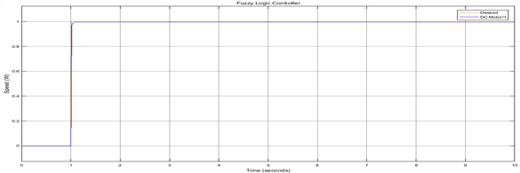
Figure 18 Simulation result of DC motor using fuzzy logic controller with disturbance.

MATLAB and SIMULINK were used to construct all of the simulations. Based on the simulation results and tables compared with and without disturbance in the case of speed control we found that the performance of the fuzzy logic controller was better than the performance of the PID controllers.

The authors declare there are no conflicts of interest.

None.

None.

1. Gubara W, Elnaim M, Babiker SF. Comparative study on the speed of DC motor using PID and FLC. In: Conference of Basic Sciences and Engineering Studies (SGCAC). IEEE.‏ 2016:24–29.
2. Almatheel YA, Abdelrahman A. Speed control of DC motor using Fuzzy Logic Controller. In: International Conference on Communication, Control, Computing and Electronics Engineering (ICCCCEE). IEEE.‏ 2017:1–8.
3. Rahman ZAS. Design a fuzzy logic controller for controlling the position of the dc motor. Int J Comput Eng Res Trends. 2017;4(7):285–289.‏
4. Ismail NL, Zakaria KA, Nazar NM, et al. DC motor speed control using a fuzzy logic controller. In: AIP Conference Proceedings. AIP Publishing LLC.‏ 2018.
5. Rajanwal K, Shakya R, Patel S, et al. Comparative analysis of PI, PID, and fuzzy logic controllers for speed control of DC motor. International Journal of Engineering Research and Technology. 2014;3(1):1319–1324.‏
6. Dökmetaş B, Akçam N. Speed Control of DC Motor Using Fuzzy Logic Application. In 4th International Symposium on Innovative Technologies in Engineering and Science (ISITES2016) 3-5 Nov 2016 Alanya/Antalya-Turkey.‏ 2016.
7. Bature AA, Muhammad M, Abdullahi AM. Design and real-time implementation of fuzzy controller for DC motor position control. International Journal of Scientific & Technology Research. 2013;2(11):254–256.‏
8. Ahmed H, Singh G, Bhardwaj V, et al. Controlling of DC Motor using Fuzzy logic controller. In Conference on advances in communication and control systems. 2013:666–670.‏
9. Kumar SB, Ali MH, Sinha A. Design and simulation of speed control of dc motor by fuzzy logic technique with Matlab/Simulink. International Journal of Scientific and Research Publications. 2014;4(7):255–299‏.
10. Soni R, Singh DBV, Pandey P, et al. Simulation of optimal speed control for a DC motor using conventional PID controller and fuzzy logic controller. International Journal of Information and Computation Technology. 2013;3(3):181–188.‏
11. Fuaâ M, Ghazaly MM. Performance comparison between PID and fuzzy logic controller in the position control system of DC servomotor. Jurnal Teknologi. 2006:1–17.‏
12. Corke P. Robotics, vision, and control: fundamental algorithms in MATLAB® second, completely revised (Vol. 118). Springer.‏ 2017.
13. Golnaraghi F, Kuo BC. Automatic control systems. McGraw-Hill Education.‏ 2017.
14. Richard C Dorf, Bishop RH. Modern control systems. Pearson Prentice Hall.‏ 2008.
15. Zadeh LA. Fuzzy sets. In Fuzzy sets, fuzzy logic, and fuzzy systems. Selected papers by Lotfi A Zadeh. 1996:394–432.‏
16. Lee CC. Fuzzy logic in control systems: fuzzy logic controller. I. IEEE Transactions on systems, man, and cybernetics. 1990;20(2):404–418.‏
17. Johnson MA, Moradi MH. PID control. Springer-Verlag London Limited.‏ 2005.
18. De Silva CW. Sensors and actuators: control system instrumentation. CRC Press.‏ 2007:699.