This paper presents a robust control technique combining adaptive sliding mode control and back–stepping methods to control a 3–DOF translational parallel robot. Dynamic modeling of the robot is accomplished using the Lagrange method. Since the derived dynamic model suffers from uncertainties and disturbances, a combination of robust techniques namely back–stepping and sliding mode controllers are applied together with adaptive control. Determination of uncertainty bounds is intransitive in the design of the proposed controller. To prove the system stability, the system model is divided into several subsystems and stability is illustrated step by step using Lyapunov criteria, then an adaptive law is obtained to estimate the uncertainties. This controller is also robust in presence of time–varying disturbances. Performance of the controller is evaluated by simulations on optimal trajectories. Trajectory planning is performed by optimization of some accuracy points using Harmony Search Algorithm (HSA) and cubic spline interpolation. Simulation results show improved performance of the proposed control technique compared to conventional feedback linearization and sliding mode techniques.

Keywords: 3–[P–2(US)] parallel robot, harmony search algorithm, adaptive back–stepping control, trajectory planning

Parallel robots are widely used in various fields of engineering and industrial applications such as, machine tools, flight simulators, earthquake simulators, medical equipment and etc. However, they have some limitations such as small and complex workspace, combination of translational and rotational motions and clearance in joints. They are also restricted by other limitations such as existence of singular points which should be studied and analysed for effective and efficient use. Therefore, their complex dynamics and forward kinematics require a very sophisticated real time control.^1-3

Since this type of robotic manipulators have a complex dynamic model, many different approaches have been applied to control them which can be classified based on the controller design methods. In this regard, classical controllers such as simple.⁴ PID controllers which are the most commonly used in industrial applications, do not need complete dynamic information of the robot. Although, these controllers usually show desirable performance in tracking of plants with linear time–invariant models, however, for robots with nonlinear dynamics, more advanced techniques such as Lyapunov based methods^5,6 or computed torque control (CTC)^7,8 improve the control performance. These methods require complete dynamic model of the robot, while the exact model is unreachable due to uncertainties. This problem restricts the performance of these nonlinear controllers. The deficiency caused by uncertainties can be compensated by adaptive back–stepping sliding mode controller which is proposed in this paper.

Sliding mode control is one of the most applicable nonlinear control strategies^9,10 which counteracts the effects of the dynamic model uncertainties. The main reason why sliding mode controller is so widely used in control of nonlinear systems is the capability of solving the two most challenging issues, stability and robustness² In order to reduce the effect of uncertainties which exist in dynamic model of parallel manipulator, a sliding mode .^11,1controller is designed in.¹³ Gracia et al.¹⁴ proposed an integrated solution based on sliding mode for trajectory tracking of a 6R robot model PUMA–560. They presented three sliding–mode algorithms for speed auto–regulation, path conditioning and redundancy resolution and finally evaluated their approach by simulations. Recently, many researchers have been characterized on designing and improving control of the parallel robots with uncertainties. Robust control based on Lyapunov’s control is the principle of most of robust and nonlinear control methods, adaptive control, sliding mode control, and combination of sliding mode and adaptive controls.^15,16 Based on the standard nonlinear adaptive methods, the controller tries to obtain specific structurally developed dynamic variable parameters; this might achieve an acceptable tracking performance and cover structuralized uncertainties and limited disturbances.¹⁷ Consequently, these factors might affect nonlinear adaptive controllers when dynamic model of the robot is not clearly known or when fast real–time control is needed.^3-5

Combined controllers of sliding mode and adaptive controls have been studied as a solution to overcome the problem of adaptive control and sliding mode. The main idea is to use adaptive control to estimate unknown parameters of the dynamic system and sliding mode control is used to overcome non–modeled dynamics and external disturbances.^18,19 However, adaptive combined control needs a parameterized liner model of the system that is analyzed and prior knowledge about the bound of uncertainty. In addition, a large number of parameters and an adaptation gain (e.g. designing parameter) corresponding with each parameter demonstrate the extent of complicacy. The problem of a robust and adaptive controller without knowledge of the bounds of uncertainties is addressed in,²⁰ where a parameterized linear model of the system is needed to design the controller. To control robot tracking in presence of uncertainties of the model and time–variable external disturbances, Notash et al.²¹ introduced a robust adaptive controller based on fuzzy logic model using neural network as a regulator tool. The controller was designed based on theoretical sliding mode control and stability of the controller was analyzed based on Lyapunov’s theory. Their findings supported very high performance and acceptable robustness in presence of disturbances. Back–stepping technique is only used to control strict feedback systems without considering the uncertain factors in practice,²² and its application is severely restricted. To gain adequate performances of control methods, many researchers have interested to the sliding mode control based on back–stepping and applied in different fields, such as chaos synchronization,^22,23 quadrotor,^24,25 motor drive,²⁶ tracking control²⁷ and etc. 

In this paper, kinematic and dynamic modeling of a 3–[P–2(US)] parallel mechanism^28,29 is investigated and equations of motion are derived via Lagrange formulation. Then, optimal trajectory planning is done based on Harmony Search Algorithm (HSA) and two trajectories are obtained by spline interpolation of optimal accuracy points in an area containing obstacles. An adaptive back–stepping sliding mode control combining both the advantages of adaptive back–stepping control and sliding mode control is used to achieve accurate control of parallel robot. In order to design of this controller, a back–stepping sliding mode controller is derived supposing that the bound of the uncertainty is well–known. Then an adaptive approach is used to estimate the uncertainties and disturbances of the derived dynamic model of the parallel robot. A Lyapunov function is used to prove the stability of the proposed controller. The proposed controller guarantees closed loop stability in spite of nonlinearities of the parallel robot. Compared with the back–stepping control scheme,³⁰ the proposed controller has the advantages of both adaptive method and robust control, which in presence of uncertainty, nonlinearity and external disturbances have a good performance. In order to overcome the existing uncertainty in this model, adaptive method is used. The main idea of back–stepping approach is to choose recursively some proper functions of state variables as fictional control inputs for lower dimension subsystems of the total system.³¹

The rest of this paper is organized as follows. In section 2, the configuration of the robot is investigated. Kinematic and dynamic modeling is depicted in section 3. In section 4, adaptive back–stepping sliding mode controller is designed. Section 5 deals with optimal path planning. Simulation results of controller implementation are reported in sections 6 and finally, conclusion is drawn in section 7.

The studied mechanism constitutes of a bottom mobile platform named end–effector, a fixed platform and three limbs. Each limb is connected to the fixed base by a prismatic joint. Prismatic joints, which are employed as actuators in this mechanism, are connected to the base from one side and connected to end–effector from other side by parallel connecting rods. In Figure 1, the assembled robot is demonstrated. Schematic presentation of the robot mechanism is depicted in Figure 2. On each limb, two universal joints are connected to two spherical joints by two connecting rods. Joints of this robot are designed in a way that only three translational motions are possible for the end–effector. Consequently, in order to prevent rotational motion of end–effector, parallelogram linkages are constructed using universal and spherical joints, thus, this robot is called 3–[P2–(US)].^28,29 The result was three translational DOF for the mechanism.

Figure 1 (a) The assembled mechanism and (b) End–effector.

Figure 2 Geometry the 3–[P2(US)] mechanism.

Inverse Kinematics

In the inverse kinematics, the goal is obtaining the actuators positions, given the end–effector position with respect to the fixed platform frame. Figure 3 demonstrates kinematic variables of a robot limb in which the end–effector position P is described in fixed platform (Frame O).

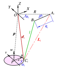
Figure 3 Kinematic variables of one of the limbs.

Referring to Figure 3, the following vector relation can be written

$L_i=q_i{e}_{A_i{B}_i}+l{e}_{B_i{C}_i}\left(i=1,2,3\right)$ (1)

Where $L_i=\overrightarrow{A_i{C}_i}$ , $e_{A_i{B}_i}$ and $e_{B_i{C}_i}$ are the unit vectors along A_iB_i and B_iC_i, respectively, and q_i represents the linear displacement of the i–th actuator.

Through rewriting Eq. (1),

$\left|L_i-q_i{e}_{A_i{B}_i}\right|=\left|l{e}_{B_i{C}_i}\right|$ (2)

After some mathematic simplification, the constraint equation is derived as:

$$\begin{gathered} {\Gamma }_i={(x-R\sin {\alpha }_i+r\sin {\alpha }_i+q_i\cos \beta \sin {\alpha }_i)}^2 \\ +{(y+R\cos {\alpha }_i-r\cos {\alpha }_i-q_i\cos \beta \cos {\alpha }_i)}^2 \\ +{(z+q_i\sin \beta )}^2-l^2=0(i=1,2,3) \end{gathered}$$                                                                                (3)

Lagrange equations

In this section, the dynamics of the robot is investigated and the dynamic model of the mechanism is derived based on the kinematic modeling which was presented in previous section. In dynamic modelling, the mass of connecting link is considered as a mass point and so waiver the joint inertia, energy dissipation and link flexibility. It is supposed that the un–modeled dynamic is evident as a disturbance in exact model. To drive the dynamic model of the robot, the Lagrange method is used. Since there are constraints on generalized coordinates in the parallel mechanism the general formulation of constrained Lagrange equations with Lagrange multipliers is considered as follows

$\frac{d}{dt}\left(\frac{\partial L}{\partial {\dot{\theta }}_j}\right)-\frac{\partial L}{\partial {\theta }_j}=Q_j+{\displaystyle \sum _{i=1}^k{\lambda }_i}\frac{\partial {\Gamma }_i}{\partial {\theta }_j}\left(j=1,\mathrm{...},6\right)$ (4)

Where ${\theta }_j$ the j–th generalized coordinate and $Q_j$ is the corresponding generalized force. Also, ${\lambda }_i$ , ${\Gamma }_i$ and k indicate the Lagrange multipliers, constraint functions and the number of system constraints, respectively. Generalized coordinates to describe the system are

$\theta =\left[\begin{array}{c}q\\ p\end{array}\right]$ (5)

Where q includes the positions of actuators (prismatic joint variables) and p includes end–effector position components. The general formulation of Lagrangian function is written as

$L(\theta ,\dot{\theta })=K(\theta ,\dot{\theta })-U(\theta )$ (6)

Where, K and U are the kinetic and potential energies of the robot, respectively. The kinetic energy term of the mechanism can be written as

$K=\frac{1}{2}{m}_1({\dot{q}}_1{}^2+{\dot{q}}_2{}^2+{\dot{q}}_3{}^2)+\frac{1}{2}{m}_2({\dot{x}}^2+{\dot{y}}^2+{\dot{z}}^2)$

$m_1=m_p+\frac{m_l}{2}{m}_2=m_e+3\left(\frac{m_l}{2}\right)$ (7)

where $m_e$ , $m_l$ , and $m_p$ are the masses of end–effector, two connecting rods, and actuators piston, respectively. Thus four concentrated moving masses constitute the kinetic energy (three masses of m₁ associated to sliding parts of actuators and one mass of m₂ associated to moving platform). According to the Figure 4, it is supposed that the masses of six connecting rods are equal and concentrated at rod ends, neglecting their rotational inertia. (Table 1)

Figure 4 Mass elements of one of the limbs.

Now, the potential energy of the mechanism can be written as

$U=-m_{1}g\sin \beta (q_1+q_2+q_3)+m_{2}gz$ (8)

Where, $\beta$ is angle of prismatic joint direction angle. Substituting Eq. (7), and (8) in Eq. (6) will result Lagrangian function as follows

$\begin{array}{l}L=\frac{1}{2}{m}_1({\dot{q}}_1{}^2+{\dot{q}}_2{}^2+{\dot{q}}_3{}^2)+\frac{1}{2}{m}_2({\dot{x}}^2+{\dot{y}}^2+{\dot{z}}^2)\\ -\left[m_{2}gz-m_{1}g\sin \beta (q_1+q_2+q_3)\right]\end{array}$ (9)

By taking partial derivatives of constraint equations used in Lagrange equations and substituting in Lagrange equation and then some simplification,³² matrix form of equations of motion is extracted as follows:

$M(\theta )\ddot{\theta }+C(\theta ,\dot{\theta })\dot{\theta }+G(\theta )=\overline{F}$ (10)

Partitioned form of the equations is written as

$\left[\begin{array}{cc}{M}_{qq}& M_{pq}\\ M_{qp}& M_{pp}\end{array}\right]\left[\begin{array}{l}\ddot{q}\\ \ddot{p}\end{array}\right]+\left[\begin{array}{cc}{C}_{qq}& C_{pq}\\ C_{qp}& C_{pp}\end{array}\right]\left[\begin{array}{l}\dot{q}\\ \dot{p}\end{array}\right]+\left[\begin{array}{l}{G}_q\\ G_p\end{array}\right]=\left[\begin{array}{l}F\\ 0\end{array}\right]$ (11)

So,

$M_{qq}\ddot{q}+M_{pq}\ddot{p}+C_{qq}\dot{q}+C_{pq}\dot{p}+G_q=F$

$M_{qp}\ddot{q}+M_{pp}\ddot{p}+C_{qp}\dot{q}+C_{pp}\dot{p}+G_p=0$ (12)

Eq. (12) is actually forward kinematics of acceleration and can be used in inverse dynamics module of control loop as follows

$\ddot{p}=-M_{pp}{}^{-1}(M_{qp}\ddot{q}+C_{qp}\dot{q}+C_{pp}\dot{p}+G_p)$ (13)

Controller design

In this section three controller is designed which is introduced in the following.

Adaptive back–stepping sliding mode control

Referring to the derived dynamic model of the proposed mechanism and defining $X_1=\theta ,X_2=\dot{\theta },X={\left[X_1{}^T,X_2{}^T\right]}^T$ , state equations of the robot can be written as:

$\{\begin{array}{l}{\dot{X}}_1=X_2\\ {\dot{X}}_2=M^{-1}\left[F-C{X}_2-G-D\right]\end{array}$ (14)

Considering as the desired trajectory of the parallel robot, the trajectory tracking error is

$e_p=q-q_d$ (15)

Virtual control variables for the parallel robot are defined as follows:

$\sigma =\epsilon e_p$ (16)

where  is a positive definite diagonal coefficient matrix. The velocity error of the system is defined as

$e_v={\dot{e}}_p+\sigma =\dot{q}-{\dot{q}}_d+\epsilon e_p$ (17)

In order to show the stability of the method, a Lyapunov function is found as follows:

$V_1(t)=\frac{1}{2}{e}_p{}^T{e}_p$ (18)

Differentiating Eq. (18) with respect to time

${\dot{V}}_1(t)=e_p{}^T{\dot{e}}_p=e_p{}^T(e_v-\epsilon e_p)=e_p{}^T{e}_v-e_p{}^T\epsilon e_p$ (19)

If $e_v=0$ , then ${\dot{V}}_1(t)\le 0$ , therefore the first subsystem of the parallel robot is stable. Differentiating Eq. (17) with respect to time gives:

${\dot{e}}_v={\ddot{e}}_p+\dot{\sigma }=\ddot{q}-{\ddot{q}}_d+\dot{\sigma }$ (20)

To indicate stability of the system, a second Lyapunov function is chosen as follows:

$V_2(t)=\frac{1}{2}\left(e_p{}^T{e}_p+S^{T}S\right)$ (21)

Where

$S=\Lambda e_p+e_v$ (22)

Where $\Lambda$ is a positive definite diagonal coefficient matrix. So, the derivation of Eq. (21) is:

${\dot{V}}_2(t)=e_p{}^T{\dot{e}}_v-e_p{}^T\epsilon e_p+S^T\left[\Lambda (e_v-\epsilon e_p)+M_{qq}{}^{-1}(F-M_{pq}\ddot{p}-C_{qq}\dot{q}-C_{pq}\dot{p}-G_q-D)-{\ddot{q}}_d+\epsilon {\dot{e}}_p\right]$ (23)

To satisfy ${\dot{V}}_2(t)\le 0$ , and stabilize the second sub–system, the controller can be designed as:

$F=M_{qq}\left[-\Lambda (e_v-\epsilon e_p)+{\ddot{q}}_d-\epsilon {\dot{e}}_p-bS\right]+M_{pq}\ddot{p}+C_{qq}\dot{q}+C_{pq}\dot{p}+G_q+\widehat{D}-\gamma M_{qq}btanh\left(\raisebox{1ex}{$S$}\!\left/ \!\raisebox{-1ex}{$\tau $}\right.\right)$ (24)

In a real–time control system, it is difficult to predict the general uncertainty D. To avoid adopting the upper bounds of D, an adaptive algorithm is applied based on back–stepping sliding mode control. By defining:

$\tilde{D}=D-\widehat{D}$ (25)

Where $\widehat{D}$ is the estimation of the general uncertainty $D$ and $\tilde{D}$ is the estimation error. Then

$\dot{\tilde{D}}=\dot{D}-\dot{\widehat{D}}=-\dot{\widehat{D}}$ (26)

The third Lyapunov function is defined as

$V_3(t)=\frac{1}{2}\left(S^{T}S+{\zeta }^{-1}{\tilde{D}}^T\tilde{D}\right)$ (27)

Where $\zeta$ is a positive constant. By taking time derivative of $V_3(t)$ and substituting Eq.(24) in it, ${\dot{V}}_3(t)$ is as follows:

${\dot{V}}_3(t)=e_p{}^T{\dot{e}}_v-e_p{}^T\epsilon e_p+S^T\left[\Lambda (e_v-\epsilon e_p)+M_{qq}{}^{-1}(F-M_{pq}\ddot{p}-C_{qq}\dot{q}-C_{pq}\dot{p}-G_q-D)-{\ddot{q}}_d+\epsilon {\dot{e}}_p\right]-{\zeta }^{-1}{\tilde{D}}^T\left(\dot{\widehat{D}}+\zeta M_{qq}{}^{-T}S\right)$ (28)

Due to ${\dot{V}}_3(t)$ should be negative, consider the adaptation law as follows:

$\dot{\widehat{D}}=-\zeta M_{qq}{}^{-T}S$ (29)

Then, the adaptive back–stepping sliding mode control law is derived as:

$F=M_{qq}\left[-\Lambda (e_v-\epsilon e_p)+{\ddot{q}}_d-\epsilon {\dot{e}}_p-bS\right]+M_{pq}\ddot{p}+C_{qq}\dot{q}+C_{pq}\dot{p}+G_q+\widehat{D}-\gamma M_{qq}btanh\left(\raisebox{1ex}{$S$}\!\left/ \!\raisebox{-1ex}{$\tau $}\right.\right)$ (30)

Where $\gamma$ is a positive definite constant and $b$ is a positive definite diagonal coefficient matrix. To avoid the enhanced chattering phenomenon, a hyperbolic tangent function is chosen in which $\tau$ is an adjustable parameter. Substituting (29) and (30) in (28), the derivative of $V_3(t)$ is as follows:

${\dot{V}}_3(t)=e_p{}^T{e}_v-e_p{}^T\epsilon e_p-S^{T}bS-\gamma S^{T}btanh\left(\raisebox{1ex}{$S$}\!\left/ \!\raisebox{-1ex}{$\tau $}\right.\right)\le e_p{}^T{e}_v-e_p{}^T\epsilon e_p-S^{T}bS$ (31)

Where

$S^{T}tanh\left(\raisebox{1ex}{$S$}\!\left/ \!\raisebox{-1ex}{$\tau $}\right.\right)³0$ , $b>0$ , $\gamma >0$ , $\tau >0$ (32)

Introducing a matrix as

$\phi =\left[\begin{array}{cc}\epsilon +{\Lambda }^{T}b\Lambda & b\Lambda -0.5I\\ b\Lambda -0.5I& b\end{array}\right]$ (33)

Then,

$\Vert \phi \Vert =b(\epsilon +\Lambda )-0.25$ (34)

By selecting the suitable parameters $b$ , $\epsilon$ and $\Lambda$ to satisfy $\Vert \phi \Vert >0$ , matrix $\phi$ is regard as the positive definite matrix. Due to

$$\begin{gathered} e^T\phi e=\left[\begin{array}{cc}{e}_p& e_v\end{array}\right]\left[\begin{array}{cc}\epsilon +{\Lambda }^{T}b\Lambda & b\Lambda -0.5I\\ b\Lambda -0.5I& b\end{array}\right]\left[\begin{array}{c}{e}_p\\ e_v\end{array}\right] \\ ={e_p}^T\epsilon e_p-{e_p}^T{e}_v+{(\Lambda e_p+e_v)}^{T}b(\Lambda e_p+e_v)={e_p}^T\epsilon e_p-{e_p}^T{e}_v+S^{T}bS \end{gathered}$$ (35)

The Eq. (31) is rewritten as

${\dot{V}}_3(t)\le -e^T\phi e$ (36)

Considering suitable values for $b$ , $\epsilon$ and $\Lambda$ then $\phi$ can be a positive definite matrix and Eq. (36) satisfies that ${\dot{V}}_3(t)\le 0$

Therefore, the globally exponential asymptotic stability of the proposed parallel robot is guaranteed. Block diagram of the proposed controller is depicted in Figure 5.

Figure 5 Block–diagram of adaptive back–stepping sliding mode control.

Inverse dynamics feedback linearization controller

Feedback linearization technique using inverse dynamics is implemented in contouring control of the proposed mechanism. Joint space variables $q$ and $\dot{q}$ are measured and taken as feedback signals to the controller. The following control law is applied in the controller.

$u={\ddot{q}}_d-k_d\dot{e}-k_{p}e$ (37)

Substituting $\ddot{q}=u$ in the inverse dynamics equations, the computed actuator forces can be determined. Block diagram of the applied control loop is illustrated in Figure 5. This control action leads to error dynamics in the form of

$\ddot{e}+k_d\dot{e}+k_{p}e=0$ (38)

Elements of the two matrices and should be chosen that the linear time–invariant error dynamics system is stable. There exists exponential convergence in the system if and re positive definite, symmetric matrices. Tuned values of the control parameters and is required for the close loop system to have desired performance in transient and steady–state responses. (Figure 6)

Figure 6 Block–diagram of feedback linearization scheme.

Sliding mode controller

A single input–single output nonlinear system can be defined as

$q^{\left(n\right)}=f(q,t)+b(q,t)F(t)$ (39)

Where,q(t) is the state vector, is the control input (in our case braking torque or pressure on the pedal) and q is the output state of the interest, f(q,t) and b(q,t) are generally nonlinear functions of time and states. The control problem is to get the state q to track a specific time–varying state $q_d(t)$ in the presence of model imprecision on f(q,t) and b(q,t).Considering the sliding surface equation of the form

$S(x,t)={\left(\frac{d}{dt}+\Lambda \right)}^2\left({\displaystyle {\int }_0^t\tilde{q}dt}\right)=\left(\frac{d^2}{d{t}^2}+2\Lambda \frac{d}{dt}+{\Lambda }^2\right)\left({\displaystyle {\int }_0^{t}edt}\right)=\dot{e}+2\Lambda e+{\Lambda }^2{\displaystyle {\int }_0^{t}edt}$ (40)

Differentiation of the sliding variable yields

$\dot{S}=\left(\ddot{q}-{\ddot{q}}_d\right)+2\Lambda \left(\dot{q}-{\dot{q}}_d\right)+{\Lambda }^2\left(q-q_d\right)$ (41)

Consider a simple second order system

$\ddot{q}=f(q,t)+F(t)\to \dot{S}=f+F-{\ddot{q}}_d+2\Lambda \left(\dot{q}-{\dot{q}}_d\right)+{\Lambda }^2\left(q-q_d\right)$ (42)

The approximation of control law $\widehat{F}(t)$ to achieve $\dot{S}=0$ is

$\widehat{F}(t)=-\widehat{f}+{\ddot{q}}_d-2\Lambda \left(\dot{q}-{\dot{q}}_d\right)-{\Lambda }^2\left(q-q_d\right)$ (43)

Which a simple solution for determining the sliding surface conditions, when the system parameters are uncertain, is the switching control law

$F(t)=\widehat{F}(t)-btanh\left(\raisebox{1ex}{$S$}\!\left/ \!\raisebox{-1ex}{$\tau $}\right.\right)$ (44)

Where k is a positive definite diagonal matrix. After some simplification, the Sliding mode control law for parallel robot is obtained as follow:

$F_{sliding}=M_{qq}({\ddot{q}}_d-2\Lambda \dot{e}-{\Lambda }^{2}e)+C_{qq}\dot{q}+G_q-M_{qq}.btanh\left(\raisebox{1ex}{$S$}\!\left/ \!\raisebox{-1ex}{$\tau $}\right.\right)$ (45)

In this section, the objective of optimal path planning is to design a trajectory for the end–effector path in an area containing some obstacles so that the trajectory is of minimum length and avoiding any collision to the obstacles. A predetermined margin is considered around the obstacles that the end–effector would keep a minimum distance with the borders of the obstacles.

To create a 2–D trajectory from starting point $P_0=(X_0,Y_0)$ to final point $P_f=(X_f,Y_f)$ in the time interval of $\left[T_0,T_f\right]$ , a number of accuracy points are considered as:

$P_i=(X_i,Y_i) at T_i (i=1,2,\mathrm{...},n)$ (46)

Where $T_i$ is the time instant at which the end–effector is planned to be located at $P_i$ . All accuracy points will be checked to be placed in the reachable workspace and far enough from singular points. End–effector trajectory is derived by cubic spline interpolation of accuracy points coordinates $X_i$ and $Y_i$ with respect to time that guarantees the continuity of velocity and acceleration. So, the trajectory curve can be obtained as,

$x_j=spline(X,T,t_j) y_j=spline(Y,T,t_j) (j=1,2,\mathrm{...},N)$ (47)

Where, N is the number of interpolated points along the curve. Spatial and time vectors are defined as,

$X=\left[X_0{X}_1{X}_2\mathrm{...}{X}_n{X}_f\right]Y=\left[Y_0{Y}_1{Y}_2\mathrm{...}{Y}_n{Y}_f\right]T=\left[T_0{T}_1{T}_2\mathrm{...}{T}_n{T}_f\right]$ (48)

The optimization problem is to obtain 2n variables consisting of $X_i$ and $Y_i$ such that the interpolated trajectory has minimum length from $P_0$ to $P_f$ and keeping the predefined margin from the obstacles. So, an objective function is considered for the optimization problem as the following form to be minimized:

$ObjFunc=\alpha C+\beta L$ (49)

Where L and C denote the trajectory length and the index of collision constraints, respectively, and the coefficients $\alpha$ and $\beta$ are the corresponding weights. The length of the trajectory is calculated by:

$L={\displaystyle \sum _{j=2}^N\sqrt{{(x_j-x_{j-1})}^2+{(y_j-y_{j-1})}^2}}$ (50)

In this research, the obstacles are considered as some circular objects. So, the index of collision constraints can be obtained as follows:

$\begin{array}{l}{d}_{j,k}=\sqrt{{(x_j-x_{C_k})}^2+{(y_j-y_{C_k})}^2}j=1,\mathrm{...},Nk=1,\mathrm{....}{n}_c\\ {\Delta }_{j,k}=max\left(1-\frac{d_{j,k}}{R_k+m},0\right)C_k=mean({\Delta }_{j,k})C={\displaystyle \sum _{k=1}^{n_c}{C}_k}\end{array}$ (51)

Where $n_c$ is the number of circular obstacles,$(X_{C_k},Y_{C_k})$ and $R_k$ are the center coordinates and the radius of the k–th obstacle, and m is the margin, respectively. The margin is considered in order to avoid the tool attached to the end–effector to collide with the obstacles. In this paper, we assume that the obstacles have been placed lower than parallel mechanism and there is no possibility for collisions of robot links with the obstacles. (Figure 7)

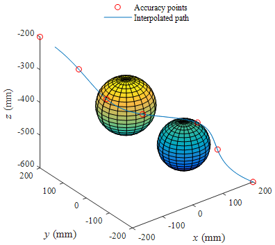
Figure 7 Optimal trajectory generated by HAS.

Same problem definition can be done for 3–D trajectory planning by introducing third coordinate Z, and solving the optimization problem with 3n variables to obtain the shortest collision–free trajectory with, for example, spherical obstacles. A harmony search algorithm is utilized for solving the optimization problem which has advantages over some other algorithms such as GA.

In this section, simulations are performed to illustrate the effectiveness of the proposed adaptive back–stepping sliding mode controller (ABS) in tracking the end–effector position. For this purpose, two trajectories are designed as a reference path and are optimized using HSA in presence of obstacles. The controller is then implemented to the robot over the designed trajectories and simulation results are obtained. Also, to indicate the robustness of the designed ABS controller, parametric uncertainties and time–varying disturbances are considered in all simulations. In order to show the outperforming of the proposed controller, their results are compared with two other controllers, a feedback linearization controller (FL) and a conventional sliding mode controller (SM). Optimal reference trajectories are tracked by the robot end–effector and discussed separately in the following. Control parameters are obtained based on harmony search algorithm. To do this, cost function which is considered is as follows:

$Obj=ITAE+\left|\dot{u}\right|$ (52)

Optimal parameters are depicted in Table 2.

Test case 1: The first trajectory is depicted in Figure 8 and tracking performances of ABS, SM, and FL controllers are shown in Figure 9, Figure 10.

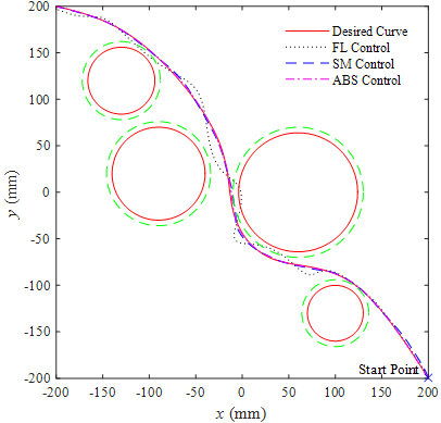
Figure 8 End–effector trajectory in the maneuver 1.

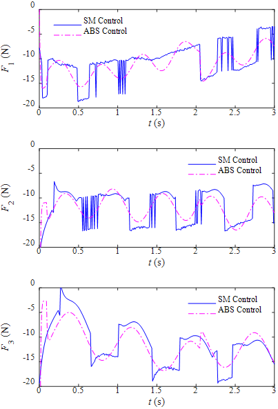
Figure 9 Control signals of proposed controller.

Figure 10 Error components of end–effector position in the maneuver 1.

As it can be seen in above figures, the proposed ABS controller provides a more reasonable tracking performance compared to the SM and FL controllers. The tracked trajectory of the ABS controller converges to the reference trajectory with a faster rate and less fluctuations than that of the SM and FL controllers. Figure 6 compares the control signal of the SM and ABS controllers which are more robust than the FL controller. As is obvious, the range of control effort in both controllers are approximately equal, however the control signal of the SM controller has larger values and intense fluctuations. Tracking errors are also indicated in Figure 10 which shows the unacceptable performance of the FL controller. The RMS of error in the SM is 2.354mm, while in the ABS method, this value is reducing to 0.7007mm.

To demonstrate the performance of the proposed controller, three criteria named as the Integral of the Time multiplied by the Absolute value of the Error (ITAE), the Integral of the Time multiplied by the Absolute value of the Squared of the Error (ITASE) and the Integral of the Absolute value of the Error (IAE) for different controller have been investigated. Three error criteria including ITAE, ITASE and IASE are considered which are defined in the following equations:

$\begin{array}{l}ITAE={\displaystyle \int \left|e(t).t\right|dt}\\ ITASE={\displaystyle \int t.{\left|e(t)\right|}^{2}dt}\\ IASE={\displaystyle \int {\left|e(t)\right|}^{2}dt}\end{array}$ (53)

Cost function may be chosen one of the defined error criteria in the paper as Eq. (53). Table 3 compares the results with different criteria. As can be seen, the results of ABS are significantly better than others.

In order to show robustness of the proposed controllers, standard deviation (STD) of error is extracted in presence of different uncertainties and depicted in Table 4.

As it can be seen, the robustness of proposed ABS controller is more than two other controllers. It should be noted that in each simulation of the controllers, external disturbances were applied.

Test case 2: A 3D spatial trajectory is considered for the second test case which is indicated from two different views in Figure 11, Figure 12. Again the tracking performances of ABS, SM, and FL controllers are simulated and shown in Figure 11, Figure 12.

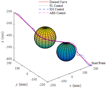
Figure 11 3D end–effector trajectory in the second maneuver.

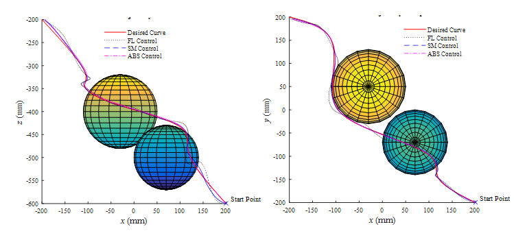
Figure 12 End–effector trajectory in the second maneuver Top view.

Figure 13 indicates the performance of the proposed ABS controller which has faster convergence compared to the SM and FL controllers. Also, less fluctuations are observed in response of the ABS controller than that of the SM and FL controllers. Tracking errors are also indicated in Figure 13 which shows the unacceptable performance of the FL controller and the 20% error reduction achieved by the ABS controller compared to the SM controller. The RMS of error in the SM is 2.652mm, while it has been reduced to 1.520mm in ABS control.

Figure 13 Error components of end–effector position in the maneuver 2.

Figure 14 compares the control signal of the SM and ABS controllers which are more robust than the FL controller. As is obvious, the range of control effort in both controllers are approximately equal, however the control signal of the SM controller has larger values and intense fluctuations. According to Figure 14 the control signal of the ABS controller has a relatively smooth behavior and no signal saturation is occurred.

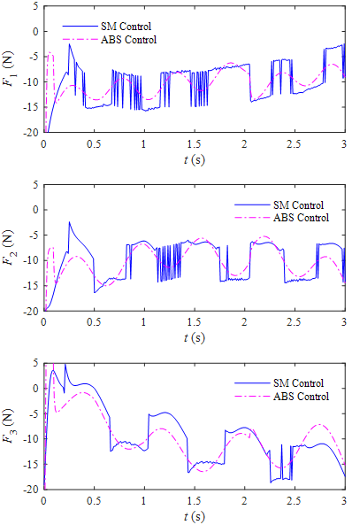
Figure 14 Control signals of proposed controller.

In order to resemble some actual conditions in laboratory setup of the mechanism, the simulations are performed in presence of disturbing forces and uncertainties considered in the dynamic model. Three sinusoidal disturbing forces with amplitudes of 2, 3, and 4 N and frequencies of 12, 10, and 8 rad/s are considered to be applied on prismatic joints. Also, a 30% deviation is parameters considered to account for uncertainties in the model. Small error components appeared in both simulations which show outperforming of the control technique in spite of the applied disturbances and uncertainties. This performance could be improved by parameter optimization of the controller. Result of the error criteria for this case is depicted in Table 5.

A three DOF translational parallel mechanism is investigated and controlled in this research. Kinematic equations are extracted based on the robot geometry and dynamic equations of motion are derived via Lagrange formulation in order to be used in robot control. To achieve minimum length and collision free trajectories for the robot motion, optimum path planning is performed using harmony search algorithm. Cubic spline interpolation is used through the obtained accuracy points in order to preserve continuity of velocity and acceleration. In order to compensate nonlinearity and uncertainties in the dynamic model, an adaptive back–stepping sliding mode control scheme is used as a robust control technique. Sliding surface equation with second order differentiation coupled with error integration is considered. Performance of the control technique is represented through two proposed maneuvers for the robot motion. Results show good achievements of the proposed controller in tracking the two desired trajectories which leads to acceptable errors even in presence of disturbances and uncertainties. In order to show the performance of proposed controller, two controllers are designed and result of the proposed controller is compared with sliding mode and feedback linearization controllers. The computed control signals are relatively smooth and saturations are not observed. According to the RMS of error in both maneuvers, the proposed controller has a better performance than the SM control.

None.

The author declares there is no conflict of interest.

1. Merlet JP. Parallel robots. 2nd ed. Netherlands: Springer; 2006. 471 p.
2. Sai LW. Robot analysis: The mechanics of serial and parallel manipulators. USA: John Wiley & Sons; 1999. 520 p.
3. Staicu Stefan. Dynamics modelling of a Stewart–based hybrid parallel robot. Advanced Robotics. 2015;29:929–938.
4. Tang L, Landers RG.Multi axis contour control the state of the art. IEEE Trans. Control Syst Technol. 2013;21(6):1997–2010.
5. Khoshdarregi MR, Tappe S, Altintas YY. Integrated five–axis trajectory shaping and contour error compensation for high–speed CNC machine tools. IEEE/ASME Trans. Mechatronics. 2014;19(6):1859–1871.
6. Wu J, Xiong Z, Ding H. Integral design of contour error model and control for biaxial system. Int J Mach Tools Manuf. 2015;89:159–169.
7. Chen SL, Tsai YC. Contouring control for multi–axis motion systems with holonomic constraints: Theory and application to a parallel system. Asian J Control. 2016;18(3): 888–898.
8. Yang J, Chen Y, Chen Y, et al. A tool path generation and contour error estimation method for four–axis serial machines. Mechatronics. 2015;31:78–88.
9. Hu C, Yao B, Wang Q. Coordinated adaptive robust contouring controller design for an industrial biaxial precision gantry. IEEE/ASME Trans Mechatronics. 2010;15(5):728–735.
10. Chen SL, Chou CY. Contouring control of robot manipulators based on equivalent errors. Asian J Control. 2014;16(3):904–914.
11. Liu S, Sun D,  Zhu C. Coordinated motion planning for multiple mobile robots along designed paths with formation requirement. IEEE/ASME Trans. Mechatronics. 2011;16(6):1021–1031.
12. Lou Y, Li Z, Zhong Y, et al. Dynamics and contouring control of a 3–DoF parallel kinematics machine. Mechatronics. 2011;21(1):215–26.
13. Garagi C D, Srinivasan K. Contouring control of Stewart platform based machine tools. Proceedings of the 2004 American Control Conference. 2004;4:3831–3838.
14. Lou Y, Chen N, Li Z. Task space based contouring control of parallel machining systems. International Conference on Intelligent Robots and Systems. 2006. p. 2047–2052.
15. Craig JJ, Hsu P, Sastry SS. Adaptive control of mechanical manipulators. The International Journal of Robotics Research. 1987;6(2):16–28.
16. Slotine JJE, Li W. Applied Nonlinear Control. USA: Prentice–Hall Inc; 1991. 259 p.
17. Seraji H. A new approach to adaptive control of manipulators. Journal of dynamic systems, measurement, and control. 1987;109(3):193–202.
18. Yao B, Bu F, Chiu GT. Non–linear adaptive robust control of electro–hydraulic systems driven by double–rod actuators. International Journal of Control. 2001;74(8):761–775.
19. Navabi M, Mirzaei H. Robust Optimal Adaptive Trajectory Tracking Control of Quadrotor Helicopter. Latin American Journal of Solids and Structures. 2017;14(6):1040–1063.
20. Gong JQ, Yao B. Adaptive robust control without knowing bounds of parameter variations. Proceedings of the 38th IEEE Decision and Control. 1999;4:3334–3339.
21. Zeinali M, Notash L. Robust adaptive neural fuzzy controller with model uncertainty estimator for manipulators. Transactions of the Canadian Society for Mechanical Engineering. 2004;28(2):197–219.
22. Yu H, Wang J, Deng B, et al. Adaptive back–stepping sliding mode control for chaos synchronization of two coupled neurons in the external electrical stimulation. Communications in Nonlinear Science and Numerical Simulation. 2012;17(3):1344–1354.
23. Li HY, Hu YA. Robust sliding–mode backstepping design for synchronization control of cross–strict feedback hyperchaotic systems with unmatched uncertainties. Communications in Nonlinear Science and Numerical Simulation. 2011;16(10):3904–3913.
24. Bouabdallah S, Siegwart R. Backstepping and sliding–mode techniques applied to an indoor micro quadrotor. Proceedings of the 2005 IEEE international conference on robotics and automation. 2005. p. 2247–2252.
25. Bouadi H, Bouchoucha M, Tadjine M. Sliding mode control based on backstepping approach for an uav type–quadrotor. Int J Appl Math Comput Sci. 2007;4(1):22–27.
26. Lin FJ, Chang CK, Huang PK. FPGA–based adaptive back–stepping sliding–mode control for linear induction motor drive. IEEE transactions on power electronics. 2007;22(4):1222–1231.
27. Choi J, Han S, Kim J. Development of a novel dynamic friction model and precise tracking control using adaptive back–stepping sliding mode controller. Mechatronics. 2006;16(2):97–104.
28. Mazare M, Taghizadeh, M, Najafi MR. Kinematic analysis and design of a 3–DOF translational parallel robot. International Journal of Automation and Computing. 2016;14(4): 432–441.
29. Mazare M, Taghizadeh, Najafi MR. Contouring control of a 3–[P2 (US)] parallel manipulator. Advanced Robotics. 2017;31(9): 496–508.
30. Faieghi MR, Delavari H, Baleanu D. A novel adaptive controller for two–degree of freedom polar robot with unknown perturbations. Communications in Nonlinear Science and Numerical Simulation. 2012;17(2):1021–1030.
31. Chiu CH, Peng YF, Lin YW. Intelligent back–stepping control for wheeled inverted pendulum. Expert Systems with Applications. 2011;38(4):3364–3371.
32. Mazare M, Taghizadeh, Najafi MR. Inverse dynamics of a 3–[P2 (US)] parallel robot.  Robotica. 2019;37(4): 708–728.