Submit manuscript...
eISSN: 2574-8092

International Robotics & Automation Journal

Correspondence:

Received: January 01, 1970 | Published: ,

Citation: DOI:

Download PDF

Abstract

In order to obtain robust and measurable data from the marine environment, citizen science projects need user-friendly tools that, during dives, autonomously gather information in an easy, low-cost and integrated way. Data collected from different devices and by different untrained divers must have good estimation of the position where the information has been acquired. With this goal, in the context of the Green Bubbles project, a novel platform, called DocuScooter has been designed and developed. DocuScooter implements all the algorithms to filter and merge data with correct timestamp and position preparing the complete mission report. After the mission, the diver can upload the report on an appropriate web service to produce a 3D documentation. In order to obtain the underwater position during the dive, a tailored device compatible with the platform is also presented. Result of the prototype of the platform and the first results of the position estimation algorithm are presented and discussed.

Keywords: citizen science, underwater robotics, underwater positioning systems, marine documentation

Abbreviations

NGC, navigation guidance and control; CS, citizen science; MPA, marine protected area; SME, small medium enterprise; COTS, component off the shelf; UKF, unscented kalman filter; GIS, geographic information system

Introduction

The preservation of the marine environment provides benefits for the whole society and constitutes a basic need for the mankind. These habitats are extremely complex systems, characterized by strong links between their physical and chemical processes and biological population. A great part of the work carried out by scientists involved in this field consists in the acquisition and analysis of robust and measurable data, in order to detect threats and take actions to contrast them. Unfortunately, this kind of activity has been proven to be very costly in terms of people and instrumentation1–3 to be carried out by a single research team with the goal to gather an amount of historical data that can allow a fully interpretation of phenomenon in this kind of environment. As a partial solution to these issues, in the last years there has been an increasing exploitation of the citizen science in marine monitoring projects, helped by the fact that in the last decades there is also a major assessing of scuba diving as a mass leisure activity, with millions of divers from all around the world. Because non-experts are involved in the research process through the citizen science, in literature there is a debate on the usefulness of this kind of researches, specifically on the quality of the data collected.4–6

Despite the advantages previously mentioned, the use of volunteers is often criticized on the basis that the information collected is unreliable as a result of either insufficient training or a lack of consistency due to the large numbers of different observers. Several research teams tried to answer to these doubts organizing training days before the missions and finding out that the data collected by the general public are consistent with those collected by the scientists.5,7,8 At a higher level of cooperation and engagement, recreational and professional divers can team up with researchers and managers to identify issues that need to be addressed, and design strategies to do so.9 Besides this aspect, the design, development and adoption of new technologies can increase the outcomes of this type of cooperation. In fact, in the recent years there is an increasing interest from the robotic community in the realization of user-friendly technologies and tools to carry out efficiently activities in the underwater environment.10–15 What the marine community is lacking is an integrated system where all the processes of acquisition, processing, analysis and output representation are gathered in a unique solution. In literature there are different examples about improving the collection or the analysis steps,16–21 where advanced low-cost techniques like structure from motion and digital photogrammetric are involved in order to estimate structural complexity of large reef areas. Anyway all these advances do not take in consideration the whole process from data acquisition to output visualization.

For this reason, a low-cost and flexible IT tool that allows professionals and/or citizen science volunteers to collect, analyze and archive different types of information simultaneously from the marine environment during a unique diving session could very helpful and useful to the marine community. Starting from this need, in the present work authors present the DocuScooter: an innovative device that allows scuba divers to automatically collect, analyze and visualize data from the ocean during their leisure activity. This latter data-processing system is called DiRAMa and the results can be stored in the most common three-dimensional formats. The system can provide ad-hoc outputs for different types of applications like data mining, Gamification and 3D printing. With the use of this system it is possible to create a wide photo database of the seabed worldwide oriented to different types of end users. In order to have more useful information that can be used for research purposes the estimation of the position of the acquired data is mandatory. In this context an additional peripheral of the Docu Scooter has been designed and developed and its operation will be introduced in this article. This component is capable to estimate the position of the diver during the mission using its on-board sensors. At the moment of writing the realization of the DocuScooter is at the first prototype step. In this paper authors present the global project, the main Mechatronic features of the developed architecture and a discussion about implemented algorithms for the position estimation. Authors are working and starting validation of the general multi-agent system structure for the scooter NGC system22 and for its hydrodynamic parameters estimation.23

The green bubbles project

The Green Bubbles project (www.greenbubbles.eu), Figure 1 funded by the EU’s H2020 Research and Innovation programme under the Marie Sklodowska-Curie grant agreement N. 643712 take care of sustainability diving. Diving nowadays has become a mass leisure activity with millions of divers all around the world. By a way it is well known that this phenomenon produces direct and indirect earnings that are able to sustain the coastal communities and the MPAs, increases the awareness to the marine environment and can help the scientific research community by interacting through the citizen science. On the other hand, a badly executed dive can lead to tangible and irreparable impacts and damages to the habitat. The main objective of the project is to maximize the benefits of the diving activities while minimizing the negative impacts to the marine environment, in order to achieve the environmental, social and economic sustainability of the whole system. One topic in particular regards the development of tailored IT tools to support citizen science projects to acquire, gather and analyze data from the marine environment.

Figure 1 The Green Bubbles logo.

DiRaMa

In order to accomplish the need of environmental monitoring in an autonomous or semi-autonomous way, in the past years Università Politecnica delle Marche team developed DiRAMa,24 a platform designed for image acquisition and three-dimensional reconstruction of submarine environments. The principal innovation brought by DiRAMa is the integration of multiple heterogeneous knowledge concerning the marine and underwater habitats using tested and reliable COTS component. This project aimed at providing greater data processing, implementing 3D reconstruction algorithms on an external server; this expands the list of possible results with a three-dimensional model of the area explored. The outcomes can be stored in the most common three-dimensional formats like PLY (Polygon File Format), OBJ + MTL, DAE (Collada), and PDF, due to the importance of letting reconstruction being modifiable with software suites of common use or open source, even directly from the mobile device employed for taking mission data. In Figure 2 a schematic representation of DiRAMa system is presented.

Figure 2 Architecture of DiRAMa.

It is possible to recognize five different components:

    1. Mobile acquisition device: any suitable technology (smartphones, tablets, smart cameras etc.) capable of sending information to DiRAMa web server.
    2. PHP/HTML5 Web server: it manages the internal user database, displays the results to end-users and communicates with the 3D Engine Module.
    3. 3D Engine module and database: it implements complex reconstruction algorithms and shares information with the Web Server. The module makes use of the database where info and elaboration results are stored.
    4. Cloud manager: it implements a notification server in order to inform the users about elaboration success or eventual errors.
    5. Home navigator: after the data elaboration is successful, end-users can download the results in order to visualize them remotely.

For further implementation details of each component, the reader can refer to.25

Docuscooter

In the context of the Green Bubbles projects Università Politecnica delle Marche (a university from Italy), Innovasub (a SME from Turkey) and Ubica (a SME from Italy) are cooperating together in order to bring innovation to the diving industry by designing and developing an innovative modular low-cost platform called DocuScooter capable to acquire heterogeneous data from the marine environment. This device is structured as an array of different devices (commercial sport cameras, lights, sensors etc.) connected to a main central unit and to an underwater Android tablet (that is optional). All the equipment is designed to equip different commercial underwater scooters that the diver can use to gather data from the marine environment while performing his leisure activity. In the recreational scuba diving there is a great employment of underwater scooters. Using this type of equipment, the capability of exploration of the marine environment by the divers is greatly increased. For this reason, the development of an add-on for an underwater scooter to gather data from this environment autonomously can be considered a great tool to help the study and monitoring of MPAs.

Aims

Main ideas behind the DocuScooter platform are:

    1. Modularity: different missions require a different sensor payload so it is necessary to have a system that allows the hot plug of different components (also during the diving activity itself) without compromising the entire system.
    2. Low cost: in order to be easily adopted by the diving industry, the platform must be low-cost and tailored to different available COTS. For example, all the cameras that can be connected to the system are sports cameras from well-known manufacturers (like GoPro or Kodak). This helps to lower the costs of the whole structure because a diver could use his/her own instrumentation.
    3. Highly extensible: it must be easy to add new compatible devices to the system with less effort as possible. To obtain this goal, in order to add a new compatible component, it is only mandatory to respect the communication protocol used to transit the data and the cable connector type.
    4. Works up to 50mt: this specification derives from the maximum depth that can be achieved by waterproof housings of commercial sports cameras.

System architecture

The architecture of the platform is presented in Figure 3. The DocuScooter is divided in three Units.

    1. User Interface Unit: It is consisting of two components: an underwater Android tablet and a subsystem. In the tablet a custom application is installed: it allows performing some basic or advanced tasks like start and following the mission, capture photos, recording video and so on. After the mission the application allows the diver to review the acquired data and upload them to the external DiRAMa service to perform data analysis. The subsystem is composed by a COTS and configurable Wi-Fi hotspot that allows the data transmission between the tablet and the rest of the system and a COTS and configurable Video Server that allows the streaming of one camera connected to the system through the screen of the tablet. It is important to notice that to perform some simple data acquisition missions this unit is optional.
    2. Motherboard unit: This unit can be considered the main communication node of the system. This unit is capable to discover, monitor and communicate with all the payload units connected to the system, receive commands from the User Interface Unit, acquire some specific data from onboard sensors (like depth and temperature) and allows to operate and monitor the state of the whole system easily through an embedded LCD screen and buttons.
    3. Payload unit: A Payload Unit is any compatible device that the diver wants to control through the User Interface Unit Android application or through the embedded screen and buttons of the Motherboard Unit. In the Figure 4 it is possible to see five different payloads (two different Wi-Fi cameras, one sensor, one light and one battery) these peripherals are a sort of intelligent devices; in fact, the single component or sensor is not directly connected to the communication bus but through a microcontroller that receives the commands and executes them.
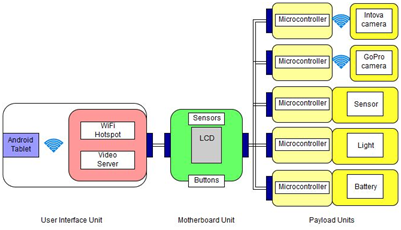
Figure 3 The DocuScooter architecture.
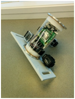
Figure 4 DocuScooter prototype.

The communication between the elements of the system (with the exception of the Android tablet that uses Wi-Fi to communicate with the system) is performed by an underwater 8 pin cable.

Underwater Position Estimator Payload Unit

As stated before, in order to obtain the position of the DocuScooter underwater while performing the survey, a specific payload unit has been designed and developed. This unit implements an estimation algorithm based on a multi-rate Unscented Kalman Filter that uses a high-rate data from an onboard IMU at fixed rate of 50Hz and slow-rate depth information from an onboard depth sensor and the position from a GPS and an USBL (when available) systems at a fixed rate of 1Hz.

Model

The state estimation is based on a discrete-time non-linear state space description:

{ x( k+1 )=f( x( k ) )+w( k ) y( k )=h( x( k ) )+v( k ) ( 1 ) MathType@MTEF@5@5@+= feaagKart1ev2aaatCvAUfeBSjuyZL2yd9gzLbvyNv2CaerbuLwBLn hiov2DGi1BTfMBaeXatLxBI9gBaerbd9wDYLwzYbItLDharqqtubsr 4rNCHbGeaGqiVCI8FfYJH8YrFfeuY=Hhbbf9v8qqaqFr0xc9pk0xbb a9q8WqFfeaY=biLkVcLq=JHqpepeea0=as0Fb9pgeaYRXxe9vr0=vr 0=vqpWqaaeaabiGaciaacaqabeaadaqaaqaaaOqaaKqbaoaaceaaea qabeaacaWG4bWaaeWaaeaacaWGRbGaey4kaSIaaGymaaGaayjkaiaa wMcaaiabg2da9iaadAgadaqadaqaaiaadIhadaqadaqaaiaadUgaai aawIcacaGLPaaaaiaawIcacaGLPaaacqGHRaWkcaWG3bWaaeWaaeaa caWGRbaacaGLOaGaayzkaaaabaGaamyEamaabmaabaGaam4AaaGaay jkaiaawMcaaiabg2da9iaadIgadaqadaqaaiaadIhadaqadaqaaiaa dUgaaiaawIcacaGLPaaaaiaawIcacaGLPaaacqGHRaWkcaWG2bWaae WaaeaacaWGRbaacaGLOaGaayzkaaaaaiaawUhaaiaacocadaqadaqa aiaaigdaaiaawIcacaGLPaaaaaa@599E@

Where the equations describe the dynamic and the measurement model of the system w(k) MathType@MTEF@5@5@+= feaagKart1ev2aaatCvAUfeBSjuyZL2yd9gzLbvyNv2CaerbuLwBLn hiov2DGi1BTfMBaeXatLxBI9gBaerbd9wDYLwzYbItLDharqqtubsr 4rNCHbGeaGqiVCI8FfYJH8YrFfeuY=Hhbbf9v8qqaqFr0xc9pk0xbb a9q8WqFfeaY=biLkVcLq=JHqpepeea0=as0Fb9pgeaYRXxe9vr0=vr 0=vqpWqaaeaabiGaciaacaqabeaadaqaaqaaaOqaaKqbakaajEhaca qIOaGaaK4AaiaajMcaaaa@39D8@ ,  is the model uncertainty and v( k ) MathType@MTEF@5@5@+= feaagKart1ev2aqatCvAUfeBSjuyZL2yd9gzLbvyNv2CaerbuLwBLn hiov2DGi1BTfMBaeXatLxBI9gBaerbd9wDYLwzYbItLDharqqtubsr 4rNCHbGeaGqiVCI8FfYJH8YrFfeuY=Hhbbf9v8qqaqFr0xc9pk0xbb a9q8WqFfeaY=biLkVcLq=JHqpepeea0=as0Fb9pgeaYRXxe9vr0=vr 0=vqpWqaaeaabiGaciaacaqabeaadaqaaqaaaOqaaKqbacbaaaaaaa aapeGaaKODamaabmaabaGaaK4AaaGaayjkaiaawMcaaaaa@3A1A@ is the measurement noise, which, for the hypothesis based on the central limit theorem, is white zero-mean Gaussian noise with respectively Q and R covariance matrices. The state is composed by position p referred to the inertial frame, velocity v and acceleration a referred to the body frame, quaternion q and angular velocity w. Moreover, the state contains the bias of accelerometer a bias MathType@MTEF@5@5@+= feaagKart1ev2aqatCvAUfeBSjuyZL2yd9gzLbvyNv2CaerbuLwBLn hiov2DGi1BTfMBaeXatLxBI9gBaerbd9wDYLwzYbItLDharqqtubsr 4rNCHbGeaGqiVCI8FfYJH8YrFfeuY=Hhbbf9v8qqaqFr0xc9pk0xbb a9q8WqFfeaY=biLkVcLq=JHqpepeea0=as0Fb9pgeaYRXxe9vr0=vr 0=vqpWqaaeaabiGaciaacaqabeaadaqaaqaaaOqaaKqbacbaaaaaaa aapeGaaKyyamaaBaaajuaibaGaaKOyaiaajMgacaqIHbGaaK4Caaqc fayabaaaaa@3C2E@  and gyroscope w bias MathType@MTEF@5@5@+= feaagKart1ev2aaatCvAUfeBSjuyZL2yd9gzLbvyNv2CaerbuLwBLn hiov2DGi1BTfMBaeXatLxBI9gBaerbd9wDYLwzYbItLDharqqtubsr 4rNCHbGeaGqiVCI8FfYJH8YrFfeuY=Hhbbf9v8qqaqFr0xc9pk0xbb a9q8WqFfeaY=biLkVcLq=JHqpepeea0=as0Fb9pgeaYRXxe9vr0=vr 0=vqpWqaaeaabiGaciaacaqabeaadaqaaqaaaOqaaKqbacbaaaaaaa aapeGaaK4Da8aadaWgaaqcfasaa8qacaqIIbGaaKyAaiaajggacaqI ZbaajuaGpaqabaaaaa@3C71@ .

x=[ p,v,a,q,w, a bias , w bias ] MathType@MTEF@5@5@+= feaagKart1ev2aaatCvAUfeBSjuyZL2yd9gzLbvyNv2CaerbuLwBLn hiov2DGi1BTfMBaeXatLxBI9gBaerbd9wDYLwzYbItLDharqqtubsr 4rNCHbGeaGqiVCI8FfYJH8YrFfeuY=Hhbbf9v8qqaqFr0xc9pk0xbb a9q8WqFfeaY=biLkVcLq=JHqpepeea0=as0Fb9pgeaYRXxe9vr0=vr 0=vqpWqaaeaabiGaciaacaqabeaadaqaaqaaaOqaaKqbakaadIhacq GH9aqpdaWadaqaaiaadchacaGGSaGaamODaiaacYcacaWGHbGaaiil aiaadghacaGGSaGaam4DaiaacYcacaWGHbWaaSbaaKqbGeaacaWGIb GaamyAaiaadggacaWGZbaajuaGbeaacaGGSaGaam4DamaaBaaajuai baGaamOyaiaadMgacaWGHbGaam4CaaqcfayabaaacaGLBbGaayzxaa aaaa@4E58@  (2)

The position dynamic26 is modeled by the equation of the uniformly accelerated motion:

f ( x( k ) ) pos = [ I 3×3 ΤR( q( k ) ) Τ 2 2 R( q( k ) ) 0 3×3 I 3×3 Τ I 3×3 0 3×3 0 3×3 I 3×3 ] [ p( k ) v( k ) a( k ) ]  ( 3 ) MathType@MTEF@5@5@+= feaagKart1ev2aaatCvAUfeBSjuyZL2yd9gzLbvyNv2CaerbuLwBLn hiov2DGi1BTfMBaeXatLxBI9gBaerbd9wDYLwzYbItLDharqqtubsr 4rNCHbGeaGqiVCI8FfYJH8YrFfeuY=Hhbbf9v8qqaqFr0xc9pk0xbb a9q8WqFfeaY=biLkVcLq=JHqpepeea0=as0Fb9pgeaYRXxe9vr0=vr 0=vqpWqaaeaabiGaciaacaqabeaadaqaaqaaaOqaaKqbakaadAgada qadaqaaiaadIhadaqadaqaaiaadUgaaiaawIcacaGLPaaaaiaawIca caGLPaaadaWgaaqcfasaaiaadchacaWGVbGaam4CaaqcfayabaGaey ypa0deaaaaaaaaa8qacaGGGcWaamWaaeaafaqabeWadaaabaGaamys amaaBaaajuaibaGaaG4maiabgEna0kaaiodaaeqaaaqcfayaaiabfs 6aujabgkci3kaadkfadaqadaqaaiaadghadaqadaqaaiaadUgaaiaa wIcacaGLPaaaaiaawIcacaGLPaaaaeaadaahaaqabeaadaWcaaqaai abfs6aunaaCaaabeqcfasaaiaaikdaaaaajuaGbaGaaGOmaaaacqGH IaYTaaGaamOuamaabmaabaGaamyCamaabmaabaGaam4AaaGaayjkai aawMcaaaGaayjkaiaawMcaaaqaaiaaicdadaWgaaqcfasaaKqbaoaa BaaajuaibaGaaG4maiabgEna0kaaiodaaeqaaaqcfayabaaabaGaam ysamaaBaaajuaibaGaaG4maiabgEna0kaaiodaaeqaaaqcfayaaiab fs6aujabgkci3kaadMeadaWgaaqcfasaaiaaiodacqGHxdaTcaaIZa aabeaaaKqbagaacaaIWaWaaSbaaKqbGeaajuaGdaWgaaqcfasaaiaa iodacqGHxdaTcaaIZaaabeaaaKqbagqaaaqaaiaaicdadaWgaaqcfa saaKqbaoaaBaaajuaibaGaaG4maiabgEna0kaaiodaaeqaaaqcfaya baaabaGaamysamaaBaaajuaibaGaaG4maiabgEna0kaaiodaaeqaaa aaaKqbakaawUfacaGLDbaacaGGGcGaeyOiGC7aamWaaeaafaqabeWa baaabaGaamiCamaabmaabaGaam4AaaGaayjkaiaawMcaaaqaaiaadA hadaqadaqaaiaadUgaaiaawIcacaGLPaaaaeaacaWGHbWaaeWaaeaa caWGRbaacaGLOaGaayzkaaaaaaGaay5waiaaw2faaiaacckacaGGJa WaaeWaaeaacaaIZaaacaGLOaGaayzkaaaaaa@95B6@

 Where I 3x3 MathType@MTEF@5@5@+= feaagKart1ev2aqatCvAUfeBSjuyZL2yd9gzLbvyNv2CaerbuLwBLn hiov2DGi1BTfMBaeXatLxBI9gBaerbd9wDYLwzYbItLDharqqtubsr 4rNCHbGeaGqiVCI8FfYJH8YrFfeuY=Hhbbf9v8qqaqFr0xc9pk0xbb a9q8WqFfeaY=biLkVcLq=JHqpepeea0=as0Fb9pgeaYRXxe9vr0=vr 0=vqpWqaaeaabiGaciaacaqabeaadaqaaqaaaOqaaKqbacbaaaaaaa aapeGaaKysa8aadaWgaaqcfasaa8qacaqIZaGaaKiEaiaajodaaKqb a+aabeaaaaa@3AF8@  and 0 3x3 MathType@MTEF@5@5@+= feaagKart1ev2aqatCvAUfeBSjuyZL2yd9gzLbvyNv2CaerbuLwBLn hiov2DGi1BTfMBaeXatLxBI9gBaerbd9wDYLwzYbItLDharqqtubsr 4rNCHbGeaGqiVCI8FfYJH8YrFfeuY=Hhbbf9v8qqaqFr0xc9pk0xbb a9q8WqFfeaY=biLkVcLq=JHqpepeea0=as0Fb9pgeaYRXxe9vr0=vr 0=vqpWqaaeaabiGaciaacaqabeaadaqaaqaaaOqaaKqbacbaaaaaaa aapeGaaKima8aadaWgaaqcfasaa8qacaqIZaGaaKiEaiaajodaa8aa beaaaaa@3A51@  are, respectively, identity and 3 all-0 matrices, and R( q( k ) ) MathType@MTEF@5@5@+= feaagKart1ev2aaatCvAUfeBSjuyZL2yd9gzLbvyNv2CaerbuLwBLn hiov2DGi1BTfMBaeXatLxBI9gBaerbd9wDYLwzYbItLDharqqtubsr 4rNCHbGeaGqiVCI8FfYJH8YrFfeuY=Hhbbf9v8qqaqFr0xc9pk0xbb a9q8WqFfeaY=biLkVcLq=JHqpepeea0=as0Fb9pgeaYRXxe9vr0=vr 0=vqpWqaaeaabiGaciaacaqabeaadaqaaqaaaOqaaKqbacbaaaaaaa aapeGaaKOuamaabmaapaqaa8qacaqIXbWaaeWaa8aabaWdbiaajUga aiaawIcacaGLPaaaaiaawIcacaGLPaaaaaa@3CB8@ is the rotation matrix from body frame to the inertial frame and is the sample time. The quaternion dynamic27 is the following:

q update  =[ cos( ω Τ 2 ) W x ω sin( ω Τ 2 ) W y ω sin( ω Τ 2 ) W z ω sin( ω Τ 2 ) ]  ( 4 ) f ( x( k ) ) quaternion = q( k )n q update   ( 5 ) MathType@MTEF@5@5@+= feaagKart1ev2aaatCvAUfeBSjuyZL2yd9gzLbvyNv2CaerbuLwBLn hiov2DGi1BTfMBaeXatLxBI9gBaerbd9wDYLwzYbItLDharqqtubsr 4rNCHbGeaGqiVCI8FfYJH8YrFfeuY=Hhbbf9v8qqaqFr0xc9pk0xbb a9q8WqFfeaY=biLkVcLq=JHqpepeea0=as0Fb9pgeaYRXxe9vr0=vr 0=vqpWqaaeaabiGaciaacaqabeaadaqaaqaaaOabaeqabaqcfaOaam yCamaaBaaajuaibaGaamyDaiaadchacaWGKbGaamyyaiaadshacaWG LbaajuaGbeaaqaaaaaaaaaWdbiaacckacqGH9aqpdaWadaqaauaabe qabqaaaaqaaiGacogacaGGVbGaai4CamaabmaabaGaeqyYdC3aaSaa aeaacqqHKoavaeaacaaIYaaaaaGaayjkaiaawMcaaaqaamaalaaaba Gaam4vamaaBaaajuaibaGaamiEaaqcfayabaaabaGaeqyYdChaaiGa cohacaGGPbGaaiOBamaabmaabaGaeqyYdC3aaSaaaeaacqqHKoavae aacaaIYaaaaaGaayjkaiaawMcaaaqaamaalaaabaGaam4vamaaBaaa juaibaGaamyEaaqcfayabaaabaGaeqyYdChaaiGacohacaGGPbGaai OBamaabmaabaGaeqyYdC3aaSaaaeaacqqHKoavaeaacaaIYaaaaaGa ayjkaiaawMcaaaqaamaalaaabaGaam4vamaaBaaajuaibaGaamOEaa qabaaajuaGbaGaeqyYdChaaiGacohacaGGPbGaaiOBamaabmaabaGa eqyYdC3aaSaaaeaacqqHKoavaeaacaaIYaaaaaGaayjkaiaawMcaaa aaaiaawUfacaGLDbaacaGGGcGaaiiOaiaacocadaqadaqaaiaaisda aiaawIcacaGLPaaaaeaacaWGMbWaaeWaaeaacaWG4bWaaeWaaeaaca WGRbaacaGLOaGaayzkaaaacaGLOaGaayzkaaWaaSbaaKqbGeaacaWG XbGaamyDaiaadggacaWG0bGaamyzaiaadkhacaWGUbGaamyAaiaad+ gacaWGUbaajuaGbeaacqGH9aqpcaGGGcGaamyCamaabmaabaGaam4A aaGaayjkaiaawMcaaiaad6gacaWGXbWaaSbaaKqbGeaacaWG1bGaam iCaiaadsgacaWGHbGaamiDaiaadwgaaKqbagqaaiaacckacaGGGcGa ai4iamaabmaabaGaaGynaaGaayjkaiaawMcaaaaaaa@9AA4@

Where ω = | W | = W x 2 + W y 2 + W z 2 MathType@MTEF@5@5@+= feaagKart1ev2aaatCvAUfeBSjuyZL2yd9gzLbvyNv2CaerbuLwBLn hiov2DGi1BTfMBaeXatLxBI9gBaerbd9wDYLwzYbItLDharqqtubsr 4rNCHbGeaGqiVCI8FfYJH8YrFfeuY=Hhbbf9v8qqaqFr0xc9pk0xbb a9q8WqFfeaY=biLkVcLq=JHqpepeea0=as0Fb9pgeaYRXxe9vr0=vr 0=vqpWqaaeaabiGaciaacaqabeaadaqaaqaaaOqaaKqbakabeM8a3b baaaaaaaaapeGaaiiOaiabg2da9iaacckadaabdaqaaiaadEfaaiaa wEa7caGLiWoacaGGGcGaeyypa0ZaaOaaaeaacaWGxbWaa0baaKqbGe aacaWG4baabaGaaGOmaaaajuaGcqGHRaWkcaWGxbWaa0baaKqbGeaa caWG5baabaGaaGOmaaaajuaGcqGHRaWkcaWGxbWaa0baaKqbGeaaca WG6baabaGaaGOmaaaaaKqbagqaaaaa@4E0C@ is the module of the angular velocity

Angular velocity, accelerometer and gyroscope bias are modeled as a linear system with  dynamic matrix. The measures are the acceleration, angular velocity from the IMU, the quaternion’s calculated from the accelerometer and magnetometer inside the IMU and the position obtained from a GPS/USBL system or a vision system. The measurement model, inclusive of gravity and bias compensation, is:

h( x( k ) )={ a( k )+a ( k ) bias +R ( q( k ) ) 1 nG W( k )+W ( k ) bias q( k ) p( k )    ( 6 ) MathType@MTEF@5@5@+= feaagKart1ev2aaatCvAUfeBSjuyZL2yd9gzLbvyNv2CaerbuLwBLn hiov2DGi1BTfMBaeXatLxBI9gBaerbd9wDYLwzYbItLDharqqtubsr 4rNCHbGeaGqiVCI8FfYJH8YrFfeuY=Hhbbf9v8qqaqFr0xc9pk0xbb a9q8WqFfeaY=biLkVcLq=JHqpepeea0=as0Fb9pgeaYRXxe9vr0=vr 0=vqpWqaaeaabiGaciaacaqabeaadaqaaqaaaOqaaKqbakaadIgada qadaqaaiaadIhadaqadaqaaiaadUgaaiaawIcacaGLPaaaaiaawIca caGLPaaacqGH9aqpdaGabaqaauaabeqaeeaaaaqaaiaadggadaqada qaaiaadUgaaiaawIcacaGLPaaacqGHRaWkcaWGHbWaaeWaaeaacaWG RbaacaGLOaGaayzkaaWaaSbaaKqbGeaacaWGIbGaamyAaiaadggaca WGZbaabeaajuaGcqGHRaWkcaWGsbWaaeWaaeaacaWGXbWaaeWaaeaa caWGRbaacaGLOaGaayzkaaaacaGLOaGaayzkaaWaaWbaaKqbGeqaba GaeyOeI0IaaGymaaaajuaGcaWGUbGaam4raaqaaiaadEfadaqadaqa aiaadUgaaiaawIcacaGLPaaacqGHRaWkcaWGxbWaaeWaaeaacaWGRb aacaGLOaGaayzkaaWaaSbaaKqbGeaacaWGIbGaamyAaiaadggacaWG ZbaabeaaaKqbagaacaWGXbWaaeWaaeaacaWGRbaacaGLOaGaayzkaa aabaGaamiCamaabmaabaGaam4AaaGaayjkaiaawMcaaaaaaiaawUha aabaaaaaaaaapeGaaiiOaiaacckacaGGGcGaai4iamaabmaabaGaaG OnaaGaayjkaiaawMcaaaaa@6F31@

Where G MathType@MTEF@5@5@+= feaagKart1ev2aqatCvAUfeBSjuyZL2yd9gzLbvyNv2CaerbuLwBLn hiov2DGi1BTfMBaeXatLxBI9gBaerbd9wDYLwzYbItLDharqqtubsr 4rNCHbGeaGqiVCI8FfYJH8YrFfeuY=Hhbbf9v8qqaqFr0xc9pk0xbb a9q8WqFfeaY=biLkVcLq=JHqpepeea0=as0Fb9pgeaYRXxe9vr0=vr 0=vqpWqaaeaabiGaciaacaqabeaadaqaaqaaaOqaaKqbacbaaaaaaa aapeGaaK4raaaa@376C@ is the gravity acceleration vector.

Unscented Kalman Filter (UKF):

The UKF28,29 is based on the propagation of the sigma points, calculated from the state and the state covariance matrix, on non-linear equations of the model. This algorithm needs to run recursively starting from the initial condition:

X ^ 0 = Ε[ X 0 ]   ( 7 ) Ρ 0  =Ε[ ( X 0 X ^ 0 ) ( X 0 X ^ 0 ) Τ ]  ( 8 ) MathType@MTEF@5@5@+= feaagKart1ev2aaatCvAUfeBSjuyZL2yd9gzLbvyNv2CaerbuLwBLn hiov2DGi1BTfMBaeXatLxBI9gBaerbd9wDYLwzYbItLDharqqtubsr 4rNCHbGeaGqiVCI8FfYJH8YrFfeuY=Hhbbf9v8qqaqFr0xc9pk0xbb a9q8WqFfeaY=biLkVcLq=JHqpepeea0=as0Fb9pgeaYRXxe9vr0=vr 0=vqpWqaaeaabiGaciaacaqabeaadaqaaqaaaOabaeqabaqcfaOabm iwayaajaWaaSbaaKqbGeaacaaIWaaajuaGbeaacqGH9aqpqaaaaaaa aaWdbiaacckacqqHvoqrdaWadaqaaiaadIfadaWgaaqcfasaaiaaic daaeqaaaqcfaOaay5waiaaw2faaiaacckacaGGGcGaaiiOaiaacoca daqadaqaaiaaiEdaaiaawIcacaGLPaaaaeaacqqHHoGudaWgaaqcfa saaiaaicdaaeqaaKqbakaacckacqGH9aqpcqqHvoqrdaWadaqaamaa bmaabaGaamiwamaaBaaajuaibaGaaGimaaqabaqcfaOaeyOeI0Iabm iwayaajaWaaSbaaKqbGeaacaaIWaaabeaaaKqbakaawIcacaGLPaaa daqadaqaaiaadIfadaWgaaqcfasaaiaaicdaaeqaaKqbakabgkHiTi qadIfagaqcamaaBaaajuaibaGaaGimaaqabaaajuaGcaGLOaGaayzk aaWaaWbaaKqbGeqabaGaeuiPdqfaaaqcfaOaay5waiaaw2faaiaacc kacaGGGcGaai4iamaabmaabaGaaGioaaGaayjkaiaawMcaaaaaaa@668F@

Where X ^ 0 MathType@MTEF@5@5@+= feaagKart1ev2aaatCvAUfeBSjuyZL2yd9gzLbvyNv2CaerbuLwBLn hiov2DGi1BTfMBaeXatLxBI9gBaerbd9wDYLwzYbItLDharqqtubsr 4rNCHbGeaGqiVCI8FfYJH8YrFfeuY=Hhbbf9v8qqaqFr0xc9pk0xbb a9q8WqFfeaY=biLkVcLq=JHqpepeea0=as0Fb9pgeaYRXxe9vr0=vr 0=vqpWqaaeaabiGaciaacaqabeaadaqaaqaaaOqaaKqbakqadIfaga qcamaaBaaajuaibaGaaGimaaqcfayabaaaaa@38FD@ the expected value of initial state is, P 0 MathType@MTEF@5@5@+= feaagKart1ev2aaatCvAUfeBSjuyZL2yd9gzLbvyNv2CaerbuLwBLn hiov2DGi1BTfMBaeXatLxBI9gBaerbd9wDYLwzYbItLDharqqtubsr 4rNCHbGeaGqiVCI8FfYJH8YrFfeuY=Hhbbf9v8qqaqFr0xc9pk0xbb a9q8WqFfeaY=biLkVcLq=JHqpepeea0=as0Fb9pgeaYRXxe9vr0=vr 0=vqpWqaaeaabiGaciaacaqabeaadaqaaqaaaOqaaKqbakaadcfada Wgaaqcfasaaiaaicdaaeqaaaaa@3857@ is the covariance matrix related to the initial state error. Three scaling parameters α,β,κ MathType@MTEF@5@5@+= feaagKart1ev2aaatCvAUfeBSjuyZL2yd9gzLbvyNv2CaerbuLwBLn hiov2DGi1BTfMBaeXatLxBI9gBaerbd9wDYLwzYbItLDharqqtubsr 4rNCHbGeaGqiVCI8FfYJH8YrFfeuY=Hhbbf9v8qqaqFr0xc9pk0xbb a9q8WqFfeaY=biLkVcLq=JHqpepeea0=as0Fb9pgeaYRXxe9vr0=vr 0=vqpWqaaeaabiGaciaacaqabeaadaqaaqaaaOqaaKqbakaajg7aca qISaGaaKOSdiaajYcacaqI6oaaaa@3BAE@ and the state dimension L are used to calculate the fixed weights λ, η 0 m , η 0 c , η i c MathType@MTEF@5@5@+= feaagKart1ev2aaatCvAUfeBSjuyZL2yd9gzLbvyNv2CaerbuLwBLn hiov2DGi1BTfMBaeXatLxBI9gBaerbd9wDYLwzYbItLDharqqtubsr 4rNCHbGeaGqiVCI8FfYJH8YrFfeuY=Hhbbf9v8qqaqFr0xc9pk0xbb a9q8WqFfeaY=biLkVcLq=JHqpepeea0=as0Fb9pgeaYRXxe9vr0=vr 0=vqpWqaaeaabiGaciaacaqabeaadaqaaqaaaOqaaKqbacbaaaaaaa aapeGaeq4UdWMaaiilaiabeE7aOnaaDaaajuaibaGaaGimaaqaaiaa d2gaaaqcfaOaaiilaiabeE7aOnaaDaaajuaibaGaaGimaaqaaiaado gaaaqcfaOaaiilaiabeE7aOnaaDaaajuaibaGaamyAaaqaaiaadoga aaaaaa@4691@

λ= α 2 ( L+k )L  ( 9 ) MathType@MTEF@5@5@+= feaagKart1ev2aaatCvAUfeBSjuyZL2yd9gzLbvyNv2CaerbuLwBLn hiov2DGi1BTfMBaeXatLxBI9gBaerbd9wDYLwzYbItLDharqqtubsr 4rNCHbGeaGqiVCI8FfYJH8YrFfeuY=Hhbbf9v8qqaqFr0xc9pk0xbb a9q8WqFfeaY=biLkVcLq=JHqpepeea0=as0Fb9pgeaYRXxe9vr0=vr 0=vqpWqaaeaabiGaciaacaqabeaadaqaaqaaaOqaaKqbacbaaaaaaa aapeGaeq4UdWMaeyypa0JaeqySde2aaWbaaKqbGeqabaGaaGOmaaaa juaGdaqadaqaaiaadYeacqGHRaWkcaWGRbaacaGLOaGaayzkaaGaey OeI0IaamitaiaacckacaGGGcGaai4iamaabmaabaGaaGyoaaGaayjk aiaawMcaaaaa@47B1@

η 0 m  = λ/( L+λ )   ( 10 ) η 0 c  = λ/( L+λ )+1 α 2 +β    ( 11 ) η i m  =  η i c  = λ/[ 2( πL+λ ) ]    ( 12 ) MathType@MTEF@5@5@+= feaagKart1ev2aaatCvAUfeBSjuyZL2yd9gzLbvyNv2CaerbuLwBLn hiov2DGi1BTfMBaeXatLxBI9gBaerbd9wDYLwzYbItLDharqqtubsr 4rNCHbGeaGqiVCI8FfYJH8YrFfeuY=Hhbbf9v8qqaqFr0xc9pk0xbb a9q8WqFfeaY=biLkVcLq=JHqpepeea0=as0Fb9pgeaYRXxe9vr0=vr 0=vqpWqaaeaabiGaciaacaqabeaadaqaaqaaaOabaeqabaqcfaOaeq 4TdG2aa0baaKqbGeaacaaIWaaabaGaamyBaaaajuaGqaaaaaaaaaWd biaacckacqGH9aqpcaGGGcGaeq4UdWMaai4lamaabmaabaGaamitai abgUcaRiabeU7aSbGaayjkaiaawMcaaiaacckacaGGGcGaaiiOaiaa cocadaqadaqaaiaaigdacaaIWaaacaGLOaGaayzkaaaabaGaeq4TdG 2aa0baaKqbGeaacaaIWaaabaGaam4yaaaajuaGcaGGGcGaeyypa0Ja aiiOaiabeU7aSjaac+cadaqadaqaaiaadYeacqGHRaWkcqaH7oaBai aawIcacaGLPaaacqGHRaWkcaaIXaGaeyOeI0IaeqySde2aaWbaaeqa juaibaGaaGOmaaaajuaGcqGHRaWkcqaHYoGycaGGGcGaaiiOaiaacc kacaGGGcGaai4iamaabmaabaGaaGymaiaaigdaaiaawIcacaGLPaaa aeaacqaH3oaAdaqhaaqcfasaaiaadMgaaeaacaWGTbaaaKqbakaacc kacqGH9aqpcaGGGcGaeq4TdG2aa0baaKqbGeaacaWGPbaabaGaam4y aaaajuaGcaGGGcGaeyypa0JaaiiOaiabeU7aSjaac+cadaWadaqaai aaikdadaqadaqaaiabec8aWjaadYeacqGHRaWkcqaH7oaBaiaawIca caGLPaaaaiaawUfacaGLDbaacaGGGcGaaiiOaiaacckacaGGGcGaai 4iamaabmaabaGaaGymaiaaikdaaiaawIcacaGLPaaaaaaa@8F39@

The sigma points are calculated from the square root of the covariance matrix.

X k  =[ X ^ k, X ^ k + L+λg Ρ k , X ^ k L+λg Ρ k ]       ( 13 ) Ρ k  =chol( Ρ k )      ( 14 ) MathType@MTEF@5@5@+= feaagKart1ev2aaatCvAUfeBSjuyZL2yd9gzLbvyNv2CaerbuLwBLn hiov2DGi1BTfMBaeXatLxBI9gBaerbd9wDYLwzYbItLDharqqtubsr 4rNCHbGeaGqiVCI8FfYJH8YrFfeuY=Hhbbf9v8qqaqFr0xc9pk0xbb a9q8WqFfeaY=biLkVcLq=JHqpepeea0=as0Fb9pgeaYRXxe9vr0=vr 0=vqpWqaaeaabiGaciaacaqabeaadaqaaqaaaOabaeqabaqcfaieaa aaaaaaa8qacaWGybWaaSbaaKqbGeaacaWGRbGaaiiOaaqabaqcfaOa eyypa0ZaamWaaeaaceWGybGbaKaadaWgaaqaaKqbGiaadUgajuaGca GGSaaabeaaceWGybGbaKaadaWgaaqcfasaaiaadUgaaeqaaKqbakab gUcaRmaakaaabaGaamitaiabgUcaRiabeU7aSjaadEgaaeqaamaaka aabaGaeuyOdi1aaSbaaKqbGeaacaWGRbaajuaGbeaaaeqaaiaacYca ceWGybGbaKaadaWgaaqcfasaaiaadUgaaeqaaKqbakabgkHiTmaaka aabaGaamitaiabgUcaRiabeU7aSjaadEgaaeqaamaakaaabaGaeuyO di1aaSbaaKqbGeaacaWGRbaajuaGbeaaaeqaaaGaay5waiaaw2faai aacckacaGGGcGaaiiOaiaacckacaGGGcGaaiiOaiaacckacaGGJaWa aeWaaeaacaaIXaGaaG4maaGaayjkaiaawMcaaaqaamaakaaabaGaeu yOdi1aaSbaaKqbGeaacaWGRbaabeaaaKqbagqaaiaacckacqGH9aqp caWGJbGaamiAaiaad+gacaWGSbWaaeWaaeaacqqHHoGudaWgaaqcfa saaiaadUgaaKqbagqaaaGaayjkaiaawMcaaiaacckacaGGGcGaaiiO aiaacckacaGGGcGaaiiOaiaacocadaqadaqaaiaaigdacaaI0aaaca GLOaGaayzkaaaaaaa@7C83@

Where chol( Ρ k ) MathType@MTEF@5@5@+= feaagKart1ev2aaatCvAUfeBSjuyZL2yd9gzLbvyNv2CaerbuLwBLn hiov2DGi1BTfMBaeXatLxBI9gBaerbd9wDYLwzYbItLDharqqtubsr 4rNCHbGeaGqiVCI8FfYJH8YrFfeuY=Hhbbf9v8qqaqFr0xc9pk0xbb a9q8WqFfeaY=biLkVcLq=JHqpepeea0=as0Fb9pgeaYRXxe9vr0=vr 0=vqpWqaaeaabiGaciaacaqabeaadaqaaqaaaOqaaKqbacbaaaaaaa aapeGaam4yaiaadIgacaWGVbGaamiBamaabmaabaGaeuyOdi1aaSba aKqbGeaacaWGRbaajuaGbeaaaiaawIcacaGLPaaaaaa@3F2A@ is the Cholesky Decomposition method

The dynamic equation is evaluated in the sigma points to calculate the predicted state X ^ k+1/k MathType@MTEF@5@5@+= feaagKart1ev2aaatCvAUfeBSjuyZL2yd9gzLbvyNv2CaerbuLwBLn hiov2DGi1BTfMBaeXatLxBI9gBaerbd9wDYLwzYbItLDharqqtubsr 4rNCHbGeaGqiVCI8FfYJH8YrFfeuY=Hhbbf9v8qqaqFr0xc9pk0xbb a9q8WqFfeaY=biLkVcLq=JHqpepeea0=as0Fb9pgeaYRXxe9vr0=vr 0=vqpWqaaeaabiGaciaacaqabeaadaqaaqaaaOqaaKqbakqadIfaga qcamaaBaaajuaibaGaam4AaiabgUcaRiaaigdacaGGVaGaam4Aaaqa baaaaa@3BE5@ and covariance matrix Ρ k+1/k MathType@MTEF@5@5@+= feaagKart1ev2aaatCvAUfeBSjuyZL2yd9gzLbvyNv2CaerbuLwBLn hiov2DGi1BTfMBaeXatLxBI9gBaerbd9wDYLwzYbItLDharqqtubsr 4rNCHbGeaGqiVCI8FfYJH8YrFfeuY=Hhbbf9v8qqaqFr0xc9pk0xbb a9q8WqFfeaY=biLkVcLq=JHqpepeea0=as0Fb9pgeaYRXxe9vr0=vr 0=vqpWqaaeaabiGaciaacaqabeaadaqaaqaaaOqaaKqbacbaaaaaaa aapeGaeuyOdi1aaSbaaKqbGeaacaWGRbGaey4kaSIaaGymaiaac+ca caWGRbaajuaGbeaaaaa@3D27@ .

X ^ k+1/k =   i=0 2L η i m f( X k i )      ( 15 ) MathType@MTEF@5@5@+= feaagKart1ev2aaatCvAUfeBSjuyZL2yd9gzLbvyNv2CaerbuLwBLn hiov2DGi1BTfMBaeXatLxBI9gBaerbd9wDYLwzYbItLDharqqtubsr 4rNCHbGeaGqiVCI8FfYJH8YrFfeuY=Hhbbf9v8qqaqFr0xc9pk0xbb a9q8WqFfeaY=biLkVcLq=JHqpepeea0=as0Fb9pgeaYRXxe9vr0=vr 0=vqpWqaaeaabiGaciaacaqabeaadaqaaqaaaOqaaKqbakqadIfaga qcamaaBaaajuaibaGaam4AaiabgUcaRiaaigdacaGGVaGaam4Aaaqa baqcfaOaeyypa0deaaaaaaaaa8qacaGGGcGaaiiOamaaqahabaGaeq 4TdG2aa0baaKqbGeaacaWGPbaabaGaamyBaaaajuaGcaWGMbWaaeWa aeaacaWGybWaa0baaKqbGeaacaWGRbaabaGaamyAaaaaaKqbakaawI cacaGLPaaaaeaacaWGPbGaeyypa0JaaGimaaqaaiaaikdacaWGmbaa cqGHris5aiaacckacaGGGcGaaiiOaiaacckacaGGGcGaai4iamaabm aabaGaaGymaiaaiwdaaiaawIcacaGLPaaaaaa@5A1B@

Ρ k+1/k = Q+ i=0 2L η i c ( ( f( X k i ) X ^ k+1/k ) ( f( X k i ) X ^ k+1/k ) T )     ( 16 ) MathType@MTEF@5@5@+= feaagKart1ev2aaatCvAUfeBSjuyZL2yd9gzLbvyNv2CaerbuLwBLn hiov2DGi1BTfMBaeXatLxBI9gBaerbd9wDYLwzYbItLDharqqtubsr 4rNCHbGeaGqiVCI8FfYJH8YrFfeuY=Hhbbf9v8qqaqFr0xc9pk0xbb a9q8WqFfeaY=biLkVcLq=JHqpepeea0=as0Fb9pgeaYRXxe9vr0=vr 0=vqpWqaaeaabiGaciaacaqabeaadaqaaqaaaOqaaKqbacbaaaaaaa aapeGaeuyOdi1aaSbaaKqbGeaacaWGRbGaey4kaSIaaGymaiaac+ca caWGRbaajuaGbeaacqGH9aqpcaGGGcGaaiyuaiabgUcaRmaaqahaba Gaeq4TdG2aa0baaKqbGeaacaWGPbaabaGaam4yaaaajuaGdaqadaqa amaabmaabaGaamOzamaabmaabaGaamiwamaaDaaajuaibaGaam4Aaa qaaiaadMgaaaaajuaGcaGLOaGaayzkaaGaeyOeI0IabmiwayaajaWa aSbaaKqbGeaacaWGRbGaey4kaSIaaGymaiaac+cacaWGRbaajuaGbe aaaiaawIcacaGLPaaadaqadaqaaiaadAgadaqadaqaaiaadIfadaqh aaqcfasaaiaadUgaaeaacaWGPbaaaaqcfaOaayjkaiaawMcaaiabgk HiTiqadIfagaqcamaaBaaajuaibaGaam4AaiabgUcaRiaaigdacaGG VaGaam4AaaqcfayabaaacaGLOaGaayzkaaWaaWbaaeqajuaibaGaam ivaaaaaKqbakaawIcacaGLPaaacaGGGcGaaiiOaiaacckacaGGGcGa aiiOaiaacocadaqadaqaaiaaigdacaaI2aaacaGLOaGaayzkaaaaba GaamyAaiabg2da9iaaicdaaeaacaaIYaGaamitaaGaeyyeIuoaaaa@7566@

The same operation is used to calculate the predicted output Y ^ k+1/k MathType@MTEF@5@5@+= feaagKart1ev2aaatCvAUfeBSjuyZL2yd9gzLbvyNv2CaerbuLwBLn hiov2DGi1BTfMBaeXatLxBI9gBaerbd9wDYLwzYbItLDharqqtubsr 4rNCHbGeaGqiVCI8FfYJH8YrFfeuY=Hhbbf9v8qqaqFr0xc9pk0xbb a9q8WqFfeaY=biLkVcLq=JHqpepeea0=as0Fb9pgeaYRXxe9vr0=vr 0=vqpWqaaeaabiGaciaacaqabeaadaqaaqaaaOqaaKqbakqadMfaga qcamaaBaaajuaibaGaam4AaiabgUcaRiaaigdacaGGVaGaam4Aaaqa baaaaa@3BE6@ and covariance Ρ k yy MathType@MTEF@5@5@+= feaagKart1ev2aaatCvAUfeBSjuyZL2yd9gzLbvyNv2CaerbuLwBLn hiov2DGi1BTfMBaeXatLxBI9gBaerbd9wDYLwzYbItLDharqqtubsr 4rNCHbGeaGqiVCI8FfYJH8YrFfeuY=Hhbbf9v8qqaqFr0xc9pk0xbb a9q8WqFfeaY=biLkVcLq=JHqpepeea0=as0Fb9pgeaYRXxe9vr0=vr 0=vqpWqaaeaabiGaciaacaqabeaadaqaaqaaaOqaaKqbakabfg6asn aaDaaajuaibaGaam4AaaqaaiaadMhacaWG5baaaaaa@3B36@

Y ^ k+1/k = i=0 2L η i m h( f( X k i ) )          ( 17 ) MathType@MTEF@5@5@+= feaagKart1ev2aaatCvAUfeBSjuyZL2yd9gzLbvyNv2CaerbuLwBLn hiov2DGi1BTfMBaeXatLxBI9gBaerbd9wDYLwzYbItLDharqqtubsr 4rNCHbGeaGqiVCI8FfYJH8YrFfeuY=Hhbbf9v8qqaqFr0xc9pk0xbb a9q8WqFfeaY=biLkVcLq=JHqpepeea0=as0Fb9pgeaYRXxe9vr0=vr 0=vqpWqaaeaabiGaciaacaqabeaadaqaaqaaaOqaaKqbakqadMfaga qcamaaBaaajuaibaGaam4AaiabgUcaRiaaigdacaGGVaGaam4Aaaqa baqcfaOaeyypa0ZaaabCaeaacqaH3oaAdaqhaaqcfasaaiaadMgaae aacaWGTbaaaaqcfayaaiaadMgacqGH9aqpcaaIWaaabaGaaGOmaiaa dYeaaiabggHiLdGaamiAamaabmaabaGaamOzamaabmaabaGaamiwam aaDaaajuaibaGaam4AaaqaaiaadMgaaaaajuaGcaGLOaGaayzkaaaa caGLOaGaayzkaaaeaaaaaaaaa8qacaGGGcGaaiiOaiaacckacaGGGc GaaiiOaiaacckacaGGGcGaaiiOaiaacckacaGGGcGaai4iamaabmaa baGaaGymaiaaiEdaaiaawIcacaGLPaaaaaa@6000@

Ρ k yy = R+ i=0 2L η i c ( h( f( X k i ) ) Y ^ k+1/k ) ( h( f( X k i ) ) Y ^ k+1/k ) T     ( 18 ) MathType@MTEF@5@5@+= feaagKart1ev2aaatCvAUfeBSjuyZL2yd9gzLbvyNv2CaerbuLwBLn hiov2DGi1BTfMBaeXatLxBI9gBaerbd9wDYLwzYbItLDharqqtubsr 4rNCHbGeaGqiVCI8FfYJH8YrFfeuY=Hhbbf9v8qqaqFr0xc9pk0xbb a9q8WqFfeaY=biLkVcLq=JHqpepeea0=as0Fb9pgeaYRXxe9vr0=vr 0=vqpWqaaeaabiGaciaacaqabeaadaqaaqaaaOqaaKqbakabfg6asn aaDaaajuaibaGaam4AaaqaaiaadMhacaWG5baaaKqbakabg2da9aba aaaaaaaapeGaaiiOaiaadkfacqGHRaWkdaaeWbqaaiabeE7aOnaaDa aajuaibaGaamyAaaqaaiaadogaaaaajuaGbaGaamyAaiabg2da9iaa icdaaeaacaaIYaGaamitaaGaeyyeIuoadaqadaqaaiaadIgadaqada qaaiaadAgadaqadaqaaiaadIfadaqhaaqcfasaaiaadUgaaeaacaWG PbaaaaqcfaOaayjkaiaawMcaaaGaayjkaiaawMcaaiabgkHiTiqadM fagaqcamaaBaaajuaibaGaam4AaiabgUcaRiaaigdacaGGVaGaam4A aaqcfayabaaacaGLOaGaayzkaaWaaeWaaeaacaWGObWaaeWaaeaaca WGMbWaaeWaaeaacaWGybWaa0baaKqbGeaacaWGRbaabaGaamyAaaaa aKqbakaawIcacaGLPaaaaiaawIcacaGLPaaacqGHsislceWGzbGbaK aadaWgaaqcfasaaiaadUgacqGHRaWkcaaIXaGaai4laiaadUgaaKqb agqaaaGaayjkaiaawMcaamaaCaaabeqcfasaaiaadsfaaaqcfaOaai iOaiaacckacaGGGcGaaiiOaiaacocadaqadaqaaiaaigdacaaI4aaa caGLOaGaayzkaaaaaa@7668@

The Cross Covariance of the state and of the output vector Ρ k xy MathType@MTEF@5@5@+= feaagKart1ev2aaatCvAUfeBSjuyZL2yd9gzLbvyNv2CaerbuLwBLn hiov2DGi1BTfMBaeXatLxBI9gBaerbd9wDYLwzYbItLDharqqtubsr 4rNCHbGeaGqiVCI8FfYJH8YrFfeuY=Hhbbf9v8qqaqFr0xc9pk0xbb a9q8WqFfeaY=biLkVcLq=JHqpepeea0=as0Fb9pgeaYRXxe9vr0=vr 0=vqpWqaaeaabiGaciaacaqabeaadaqaaqaaaOqaaKqbakabfg6asn aaDaaajuaibaGaam4AaaqaaiaadIhacaWG5baaaaaa@3B35@ is calculated as:

Ρ k xy = R+ i=0 2L η i c ( h( f( X k i ) ) X ^ k+1/k ) ( h( f( X k i ) ) Y ^ k+1/k ) T     ( 19 ) MathType@MTEF@5@5@+= feaagKart1ev2aaatCvAUfeBSjuyZL2yd9gzLbvyNv2CaerbuLwBLn hiov2DGi1BTfMBaeXatLxBI9gBaerbd9wDYLwzYbItLDharqqtubsr 4rNCHbGeaGqiVCI8FfYJH8YrFfeuY=Hhbbf9v8qqaqFr0xc9pk0xbb a9q8WqFfeaY=biLkVcLq=JHqpepeea0=as0Fb9pgeaYRXxe9vr0=vr 0=vqpWqaaeaabiGaciaacaqabeaadaqaaqaaaOqaaKqbakabfg6asn aaDaaajuaibaGaam4AaaqaaiaadIhacaWG5baaaKqbakabg2da9aba aaaaaaaapeGaaiiOaiaadkfacqGHRaWkdaaeWbqaaiabeE7aOnaaDa aajuaibaGaamyAaaqaaiaadogaaaaajuaGbaGaamyAaiabg2da9iaa icdaaeaacaaIYaGaamitaaGaeyyeIuoadaqadaqaaiaadIgadaqada qaaiaadAgadaqadaqaaiaadIfadaqhaaqcfasaaiaadUgaaeaacaWG PbaaaaqcfaOaayjkaiaawMcaaaGaayjkaiaawMcaaiabgkHiTiqadI fagaqcamaaBaaajuaibaGaam4AaiabgUcaRiaaigdacaGGVaGaam4A aaqcfayabaaacaGLOaGaayzkaaWaaeWaaeaacaWGObWaaeWaaeaaca WGMbWaaeWaaeaacaWGybWaa0baaKqbGeaacaWGRbaabaGaamyAaaaa aKqbakaawIcacaGLPaaaaiaawIcacaGLPaaacqGHsislceWGzbGbaK aadaWgaaqcfasaaiaadUgacqGHRaWkcaaIXaGaai4laiaadUgaaKqb agqaaaGaayjkaiaawMcaamaaCaaabeqcfasaaiaadsfaaaqcfaOaai iOaiaacckacaGGGcGaaiiOaiaacocadaqadaqaaiaaigdacaaI5aaa caGLOaGaayzkaaaaaa@7667@

The Kalman gain Κ k MathType@MTEF@5@5@+= feaagKart1ev2aaatCvAUfeBSjuyZL2yd9gzLbvyNv2CaerbuLwBLn hiov2DGi1BTfMBaeXatLxBI9gBaerbd9wDYLwzYbItLDharqqtubsr 4rNCHbGeaGqiVCI8FfYJH8YrFfeuY=Hhbbf9v8qqaqFr0xc9pk0xbb a9q8WqFfeaY=biLkVcLq=JHqpepeea0=as0Fb9pgeaYRXxe9vr0=vr 0=vqpWqaaeaabiGaciaacaqabeaadaqaaqaaaOqaaKqbakabfQ5aln aaBaaajuaibaGaam4Aaaqabaaaaa@392B@  is calculated from the Covariance and Cross Covariance matrices:

Κ k = Ρ k xy ( Ρ k yy ) 1        ( 20 ) MathType@MTEF@5@5@+= feaagKart1ev2aaatCvAUfeBSjuyZL2yd9gzLbvyNv2CaerbuLwBLn hiov2DGi1BTfMBaeXatLxBI9gBaerbd9wDYLwzYbItLDharqqtubsr 4rNCHbGeaGqiVCI8FfYJH8YrFfeuY=Hhbbf9v8qqaqFr0xc9pk0xbb a9q8WqFfeaY=biLkVcLq=JHqpepeea0=as0Fb9pgeaYRXxe9vr0=vr 0=vqpWqaaeaabiGaciaacaqabeaadaqaaqaaaOqaaKqbakabfQ5aln aaBaaajuaibaGaam4AaaqabaqcfaOaeyypa0JaeuyOdi1aa0baaKqb GeaacaWGRbaabaGaamiEaiaadMhaaaqcfa4aaeWaaeaacqqHHoGuda qhaaqcfasaaiaadUgaaeaacaWG5bGaamyEaaaaaKqbakaawIcacaGL PaaadaahaaqcfasabeaacqGHsislcaaIXaaaaKqbacbaaaaaaaaape GaaiiOaiaacckacaGGGcGaaiiOaiaacckacaGGGcGaaiiOaiaacoca daqadaqaaiaaikdacaaIWaaacaGLOaGaayzkaaaaaa@5525@

Hence, the estimated state X ^ k+1 MathType@MTEF@5@5@+= feaagKart1ev2aaatCvAUfeBSjuyZL2yd9gzLbvyNv2CaerbuLwBLn hiov2DGi1BTfMBaeXatLxBI9gBaerbd9wDYLwzYbItLDharqqtubsr 4rNCHbGeaGqiVCI8FfYJH8YrFfeuY=Hhbbf9v8qqaqFr0xc9pk0xbb a9q8WqFfeaY=biLkVcLq=JHqpepeea0=as0Fb9pgeaYRXxe9vr0=vr 0=vqpWqaaeaabiGaciaacaqabeaadaqaaqaaaOqaaKqbakqadIfaga qcamaaBaaajuaibaGaam4AaiabgUcaRiaaigdaaKqbagqaaaaa@3AD0@  and error Covariance Ρ k+1 MathType@MTEF@5@5@+= feaagKart1ev2aaatCvAUfeBSjuyZL2yd9gzLbvyNv2CaerbuLwBLn hiov2DGi1BTfMBaeXatLxBI9gBaerbd9wDYLwzYbItLDharqqtubsr 4rNCHbGeaGqiVCI8FfYJH8YrFfeuY=Hhbbf9v8qqaqFr0xc9pk0xbb a9q8WqFfeaY=biLkVcLq=JHqpepeea0=as0Fb9pgeaYRXxe9vr0=vr 0=vqpWqaaeaabiGaciaacaqabeaadaqaaqaaaOqaaKqbakabfg6asn aaBaaajuaibaGaam4AaiabgUcaRiaaigdaaKqbagqaaaaa@3B64@  are calculated as:

X ^ k+1 = X ^ k+1/k + Κ k ( Y k+1 Y ^ k+1/k )      ( 21 ) MathType@MTEF@5@5@+= feaagKart1ev2aaatCvAUfeBSjuyZL2yd9gzLbvyNv2CaerbuLwBLn hiov2DGi1BTfMBaeXatLxBI9gBaerbd9wDYLwzYbItLDharqqtubsr 4rNCHbGeaGqiVCI8FfYJH8YrFfeuY=Hhbbf9v8qqaqFr0xc9pk0xbb a9q8WqFfeaY=biLkVcLq=JHqpepeea0=as0Fb9pgeaYRXxe9vr0=vr 0=vqpWqaaeaabiGaciaacaqabeaadaqaaqaaaOqaaKqbakqadIfaga qcamaaBaaajuaibaGaam4AaiabgUcaRiaaigdaaKqbagqaaiabg2da 9iqadIfagaqcamaaBaaajuaibaGaam4AaiabgUcaRiaaigdacaGGVa Gaam4AaaqcfayabaGaey4kaSIaeuOMdS0aaSbaaKqbGeaacaWGRbaa juaGbeaadaqadaqaaiaadMfadaWgaaqcfasaaiaadUgacqGHRaWkca aIXaaabeaajuaGcqGHsislceWGzbGbaKaadaWgaaqcfasaaiaadUga cqGHRaWkcaaIXaGaai4laiaadUgaaeqaaaqcfaOaayjkaiaawMcaaa baaaaaaaaapeGaaiiOaiaacckacaGGGcGaaiiOaiaacckacaGGGcGa ai4iamaabmaabaGaaGOmaiaaigdaaiaawIcacaGLPaaaaaa@5D4A@

Ρ k+1 = Ρ k+1/k + Κ k Ρ k yy Κ k T       ( 22 ) MathType@MTEF@5@5@+= feaagKart1ev2aaatCvAUfeBSjuyZL2yd9gzLbvyNv2CaerbuLwBLn hiov2DGi1BTfMBaeXatLxBI9gBaerbd9wDYLwzYbItLDharqqtubsr 4rNCHbGeaGqiVCI8FfYJH8YrFfeuY=Hhbbf9v8qqaqFr0xc9pk0xbb a9q8WqFfeaY=biLkVcLq=JHqpepeea0=as0Fb9pgeaYRXxe9vr0=vr 0=vqpWqaaeaabiGaciaacaqabeaadaqaaqaaaOqaaKqbakabfg6asn aaBaaajuaibaGaam4AaiabgUcaRiaaigdaaKqbagqaaiabg2da9iab fg6asnaaBaaajuaibaGaam4AaiabgUcaRiaaigdacaGGVaGaam4Aaa qcfayabaGaey4kaSIaeuOMdS0aaSbaaKqbGeaacaWGRbaajuaGbeaa cqqHHoGudaqhaaqcfasaaiaadUgaaeaacaWG5bGaamyEaaaajuaGcq qHAoWsdaqhaaqcfasaaiaadUgaaeaacaWGubaaaKqbacbaaaaaaaaa peGaaiiOaiaacckacaGGGcGaaiiOaiaacckacaGGGcGaai4iamaabm aabaGaaGOmaiaaikdaaiaawIcacaGLPaaaaaa@5B1F@

Preliminary tests

Presently the realization of the DocuScooter is at the first prototype step. The electronics of the User Interface Unit, the whole Motherboard unit and multiple microcontrollers of the Payload unit have been inserted in a unique watertight box in order to perform the preliminary tests. The underwater tablet that has been employed during the validation was an Alleco AllTab2. Three underwater action cameras of different brands (GoPro Hero 3 Black, Kodak PixPro Sp360 and Intova EdgeX) have been used as payloads in order to perform the 3D reconstruction. Figure 4 presents the first prototype of DocuScooter. After the system has been verified to correctly work out of water, a series of test have been conducted in water. Specifically, the system was proved in different missions by the marine biologists of Hopkins Marine Station of Stanford University in the Monterey Bay, CA. The aim of the mission was to evaluate the functionality of the system and the inspection of a semi-submerged pipe located at the bottom of the seabed. The diver was instructed to survey the pipe different times in order to have images redundancy for the 3D reconstruction process of an area of about 2 x 14 meters.

After the dive the gathered data set is uploading to the DiRAMa servers. The time for obtaining the 3D model depends mainly on two factors: the number of the photos and the quality requested. A low quality model can be available with few hours of elaboration and this means that the researchers can better organize another survey for the same day or the day after analyzing the site models obtained with the feedback. The high quality model is instead available in 1 month, together with the possibility of having also its 3D print. In Figure 5 the low quality model resulted from the mentioned missions is shown. It was obtained from the elaboration of about 200 photos in four hours. The high quality output can be produced in different formats, so manageable with different kind of software and for different kind of usages. It can be imported in virtual environments like common game engines (the authors use Unity) or common GIS (the authors use QGIS) which makes its fruition easier. In parallel to the reconstruction process, from the cameras alignment and correspondence steps, is possible to recover also the trajectory followed by the diver. An example of this output related to the pipe inspection is illustrated in Figure 6. It can be noticed that the diver started the survey from the middle of the pipe and the continued along its length. In this phase the filtering algorithm was implemented on a National Instrument MyRIO and tested on the DocuScooter which was moved only on the surface to allow acquiring the GPS data. Due to the particular nature of this test, no depth sensor has been involved in the algorithm. The IMU used during this test was an Xsens MTi-3-8A7G6, installed on center of gravity of the vehicle. The Ad fruit Ultimate GPS v3 has been used to receive the GPS signal with an active antenna. The accuracy of this sensor is about 3 meters. These two sensors have been used to feed the data to the UKF algorithm.
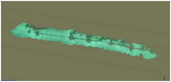
Figure 5 Low quality 3D model.
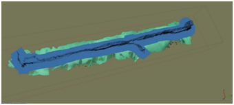
Figure 6 Path followed by the diver.

Table 1 gathers quantitative results regarding five tests that have been performed. The maximum and the mean error are related to the real GPS position. As the table shows, the algorithm is able to satisfactorily estimate the position of the device during the test. For sake of brevity only the results and graphs related to Test 1 will be analyzed and discussed. In any case, comparable considerations could be done with the data acquired during the other tests.

Test Time (s)

Max Error (m)

Mean Error (m)

Test 1

421

0.9154

0.0966

Test 2

877

0.7151

0.1034

Test 3

244

0.8519

0.1466

Test 4

414

0.7268

0.0797

Test 5

719

0.6153

0.0847

Table 1 Quantitative results of the five tests performed

It is possible to observe that only in the first seconds the filtered position doesn’t track perfectly the GPS because the accelerometer bias wasn’t compensated, as confirmed by position error (Figure 8). Confirming a good behavior of the UKF, Figure 9 shows the track of the estimated heading compared to heading computed by the GPS. In this case the gyro bias is very small, so the filter works well also in the first’s instants.
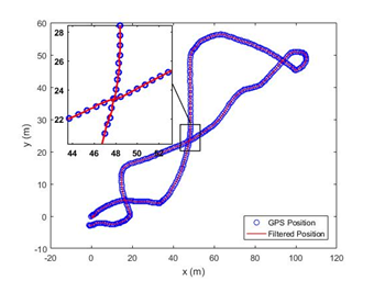
Figure 7 GPS and filtered position Figure 7 show device position measured from GPS and filtered by the UKF algorithm.
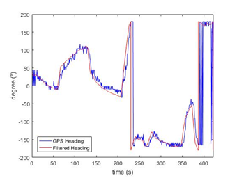
Figure 8 Position error.

Figure 9 GPS and filtered heading.

Conclusion

In this paper we presented a novel platform tailored to acquire process and visualize data in an integrated way, despite the state of the art that is actually present in literature. Due to the ease of use, DocuScooter platform could be easily employed by the marine citizen science increasing in this way the quantity of data for the scientific analysis while having fun during a diving mission. The designed and developed algorithm has been proven to be robust enough to be implemented in the final version of the DocuScooter. Further development of the DocuScooter will be implementation and validation of a general multi-agent system structure for the NGC system in order to allow auto-piloting. To improving the energy efficiency of the scooter, test implying the hydrodynamic parameters identification will be designed and performed.

Acknowledgements

This project has received funding from the European Unions’s Horizon 2020 research and innovation program under the Marie Sklodowska-Curie grant agreement No 643712.

Conflict of interest

The author declares no conflict of interest

References

  1. Danielsen F, Burgess ND, Balmford A. Monitoring matters: examining the potential of locally-based approaches. Biodiversity & Conservation. 2005;14(11):2507–2542.
  2. Hochachka WM, Fink D, Hutchinson RA, et al. Data-intensive science applied to broad-scale citizen science. Trends Ecol Evol. 2012;27(2):130–137.
  3. Hodgson G. A global assessment of human effects on coral reefs. Marine Pollution Bulletin. 1999;38(5):345–355.
  4. Fore LS, Paulsen K, O Laughlin K. Assessing the performance of volunteers in monitoring streams. Freshwater Biology. 2001;46(1):109–123.
  5. Van der Velde T, Milton DA, Lawson TJ, et al. Comparison of marine debris data collected by researchers and citizen scientists: Is citizen science data worth the effort. Biological Conservation. 2016. p. 1–12.
  6. Vann-Sander S, Clifton J, Harvey E. Can citizen science work? Perceptions of the role and utility of citizen science in a marine policy and management context. Marine Policy. 2016;72:82–93.
  7. Foster Smith J, Evans SM. The value of marine ecological data collected by volunteers. Biological Conservation. 2003;113(2):199–213.
  8. Delaney DG, Sperling CD, Adams CS, et al. Marine invasive species: validation of citizen science and implications for national monitoring networks. Biological Invasions. 2008;10(1):117–128.
  9. Cerrano C, Milanese M, Ponti M. Diving for science-science for diving: volunteer scuba divers support science and conservation in the Mediterranean Sea: Citizen Science for Mediterranean MPAs. Aquatic conservation marine and freshwater ecosystems; 2016.
  10. Scaradozzi D, Conte G, De Capua GP, et al. Innovative technology for studying growth areas of posidonia oceanic. IEEE workshop on environmental, Energy, and Structural monitoring systems (EESMS); 2009.
  11. Zapata-Ramírez PA, Scaradozzi D, Sorbi L, et al. Innovative study methods for the Mediterranean coralligenous habitats. Advances in Oceanography and Limnology. 2013;4(2):102–119.
  12. Zapata-Ramírez PA, Huete-Stauffer C Scaradozzi D, et al. Testing methods to support management decisions in coralliferous and cave environments. A case study at Portofino MPA. Mar Environ Res. 2016;118:45–56.
  13. Williams SB, Pizarro OR, Jakuba MV, et al. Monitoring of benthic reference sites: using an autonomous underwater vehicle. IEEE Robotics & Automation Magazine. 2012;19(1):73–84.
  14. Scaradozzi D, Conte G, Sorbi L. Assisted guidance system for Micro ROV in underwater data gathering missions. 20th mediterranean conference on control and automation, MED 2012 Conference Proceedings; USA: Springer; 2012. p. 1373–1378.
  15. Puillat I, Prevosto M, Mercier H, et al. Time series analysis of marine data: A key knowledge at the crossroads of marine sciences. Journal of Marine Systems. 2014;130:1–3.
  16. Ferrari R, Bryson M, Bridge T, et al. Quantifying the response of structural complexity and community composition to environmental change in marine communities. Global change biology. 2016;22(5):1965–1975.
  17. Figueira W, Ferrari R, Weatherby E, et al. Accuracy and precision of habitat structural complexity metrics derived from underwater photogrammetric. Remote Sens. 2015;7(12):16883–16900.
  18. McCarthy J. Multi-image photogrammetry as a practical tool for cultural heritage survey and community engagement. Journal of Archaeological Science. 2014;43:175–185.
  19. Storlazzi CD, Dartnell P, Hatcher GA, et al. End of the chain? Rugosity and fine-scale bathymetry from existing underwater digital imagery using structure-from-motion (SfM) technology. Coral Reefs. 2016;35(3):889–894.
  20. Westobya MJ, Brasingtonb J, Glassera NF, et al. Structure-from-Motion’photogrammetry: A low-cost, effective tool for geoscience applications. Geomorphology. 2012;179:300–314.
  21. Matthew W, Dunning S, Allan M, et al. From an 'ice-see' perspective: The current use, potential and limitations of Structure-from-Motion photogrammetry for cryospheric applications. Geophysical Research Abstracts. 2016;18:1.
  22. Morganti G, Perdon AM, Conte G, et al. Multi-agent system theory for modelling a home automation system. International Work-Conference on Artificial Neural Networks. 2009;5517LNCS (Part 1):585–593.
  23. Conte G, Zanoli SM, Scaradozzi D, et al. Evaluation of hydrodynamics parameters of a UUV. A preliminary study. International Symposium on Control, Communications and Signal Processing; USA: Springer; 2004. p. 545–548.
  24. Sorbi L, Zoppini F, Zingaretti S, et al. Robotic tools and techniques for improving research in underwater delicate environment. Marine Technology Society Journal. 2015;49(5):6–17(12).
  25. Scaradozzi D, Sorbi L, Zoppini F, et al. Innovative strategy and process for underwater data gathering and results elaboration. 22nd mediterranean conference on control and automation (MED); Italy: IEEE; 2014.
  26. Caron F, Duflos E, Pomorski D, et al. GPS/IMU data fusion using multisensor Kalman filtering: introduction of contextual aspects. Information Fusion. 2006;7(2):221–230.
  27. Armesto L, Chroust S, Vincze M, et al. Multi-rate fusion with vision and inertial sensors. Robotics and Automation. 2004;1:193–199.
  28. Zhao G, Fu K, Chen S, et al. Scaled UKF with reduced sigma points particle filter for a red shift navigation system, 34th Chinese control conference (CCC); China: IEEE; 2015. p. 5218–5223.
  29. Lv H, Wei G, Ding Z. UKF-Based for sensorless brushless DC motor control international conference on mechatronics and control (ICMC); China: IEEE; 2014. p. 199–203.
Creative Commons Attribution License

© . This is an open access article distributed under the terms of the, which permits unrestricted use, distribution, and build upon your work non-commercially.