Fluid flow in low permeability porous media does not obey Darcy's law anymore, so traditional well testing interpretation methods may cause the error in estimation of low permeability oil reservoir parameters. This paper describes problems encountered when analyzing transient pressure tests in ultra-low permeability oil reservoir. Based on the new model, the theoretical well test model for dual-porosity media in low permeability oil reservoirs with complex fractures was derived, allowing the influencial analysis of non-Darcy's effect. The model was created by analytical solution and numerical approach. Besides, the curves for the pressure responses were plotted. The effects of parameters including fracture width, fracture length and the position of the fracture were fully investigated. The advantage of the solution is that it is easy to incorporate storability ratio and skin factor. Also, it can simplify the computation process and make enhance the efficiency. Sensitivity analysis shows that non-Darcy flow mainly affects the transition section between the pure wellbore storage and radial flow region, and the pressure derivative curves exhibit a gentle transition region compared with the Darcy's flow. These curves provide a better way to characterize the well testing pressure response for ultra-low permeability oil reservoir.

At present, the oil exploration and development in China faces two severe problems--high water cut and low permeability. Plenty of studies have been done on pressure propagation in low permeability reservoirs, leading to some significant progress. Pascal¹ applied the numerical integration methods, which is a finite difference method, to solve the problem of consolidation of geotechnical engineering for the first time by considering the pressure gradient. Yan Qinglai² summed up the laboratory experimental results of single phase flow characteristics in low permeability reservoirs and flow curves' characteristics of distilled water, low saline water and simulated crude oil, which were made to flow through artificial and natural cores. Huang Yan zhang³ derived mathematical equation of percolation for low permeability reservoir and studied the percolation feature and regularity of oil and water. Yao Yuedong⁴ analyzed the experimental data of fluid flow in porous core with low permeability and plotted typical logarithmic curves. At the same time, three typical transient flow models for low-permeability reservoirs were built and the approximate analytical solutions in Laplace space were obtained. Zhu Shengju⁵ used the steady state replacement method to study the propagation of pressure wave of unsteady flow of elastic fluid in low permeability reservoirs. Based on the percolation features of low permeability reservoirs, Yang Qingli⁶ put forward the continuous model of nonlinear percolation and derived the equation of pressure distribution and moving boundary spreading for unsteady state flow. Based on the theory of pressure wave ellipse constant pressure surface spreading, Qiao Wei⁷ deduced the relationship between pressure wave propagation time and elliptic mobile boundary for plane ellipse radial flow and spheroid centripetal flow of fracturing well in low permeability reservoir, and compared it to the laws of pressure wave spreading of plane parallel flow, plane radial flow and spherical centripetal flow.

Model description

Figure 1 shows the model of a finite large homogeneous low permeability reservoir, with the thickness of h. The average permeability is k under the reservoir pressure. Due to the presence of starting pressure gradient in low permeability reservoir, the pressure continues to spread deeply to the geological formations with time going on. According to the low permeability theory, the following assumptions were made for the fluid flow in the circumstances:

Figure 1: A physical model of the plane radial diagram.

The formation of the reservoir is isopachous, bounded and heterogeneous.

1. Before the production wells produce, the reservoir pressure is equal to the original formation pressure.
2. The fluid of the reservoir is slightly compressible, and flows with unsteady single-phase flow instability.
3. The effect of the permeability of the pressure-sensitive is not considered, and the fluid of porous media porosity and viscosity are regarded as constant.
4. The reservoir fluid flow within a limited range to the wellbore. Radial flow of fluid occurs

Non-fracture model derivation

Being different from high permeability reservoirs, low permeability reservoir is not in line with the classical Darcy's law, and the most obvious feature of low permeability reservoir is the presence of starting pressure gradient, and the seepage law can be written and the following equation.⁸

$v=\frac{k}{\mu }(1-\frac{c_1}{\frac{dp}{dr}}-\frac{c_2}{\frac{dp}{dr}-c_3})\frac{dp}{dr}$ (1)

Where k is the reservoir effective permeability and µ is the oil viscosity at reservoir conditions.
If $c_1=c_2=0$ , the equation (1) will be Darcy's model, if $c_1\ne 0,c_2=0$ , the equation (1) will be quasi start-up pressure gradient model (quasi-linear flow), if $c_1\ne 0,c_2\ne 0$ , the equation (1) will be three-parameter continuous model, and if $c_1\ne 0,c_2\ne 0,c_3\ne 0$ , different curves can be achieved.⁸
Flow velocity at any position can be written as:

$v=\frac{Bq}{A}$ (2)

$A=wh$ (3)

Where r is the drainage radius and h is the reservoir effective thickness. B is the formation volume factor of crude oil under original pressure. Q is the ground crude oil production, and A is the seepage area.

Substitute equation (2) and (3) into equation (1), by ignoring high order infinitely small quantity, (1) can be rewritten as

$\{\begin{array}{l}r{\left(\frac{dp}{dr}\right)}^2-[r(c_1+c_2+c_3)+\frac{Bq\mu }{2\pi kh}]\frac{dp}{dr}+\frac{c_{3}Bq\mu }{2\pi kh}=0\\ {p|}_{r=r_w}=p_{wf},{p|}_{r=r_{\text{e}}}=p_e\end{array}$ (4)

By solving equation (4), we have

$\frac{dp}{dx}=\frac{c_1+c_2+c_3}{2}+\frac{Bq\mu }{4\pi khr}+\frac{\sqrt{{[r(c_1+c_2+c_3)+\frac{Bq\mu }{2\pi kh}]}^2-\frac{2r{c}_{3}Bq\mu }{\pi kh}}}{2r}$ (5)

Steady successive substitution method noted that in unsteady flow, pressure distribution can be approximated as a steady flow process at a certain time, and the pressure spread boundary radius is the function of time t, which is represented by r(t). By integrating equation (5), bottom whole pressure and pressure distribution at any time can be obtained.

$p(r)=p_{wf}+{\begin{array}{l}\frac{1}{C_1}[N{C}_{1}f(r)-N^2{C}_{1}ln\frac{N^2+rN{C}_2+Nf(r)}{0.5r}\\ +N^2{C}_{2}ln\frac{N(c_1+c_2-c_3)+r{C}_1{}^2+C_{1}f(r)}{C_1}]\end{array}|}_{r_w}^{r(t)}$ (6)

Where

$f(r)=\sqrt{{[r(c_1+c_2+c_3)+N]}^2-4c_{3}N}$ (7)

$C_1=c_1+c_2+c_3$ , $C_2=c_1+c_2-c_3$ (8)

$N=\frac{Bq\mu }{2\pi kh}$ (9)

The situation of p(r) is complicated and it is difficult for the follow-up studies on pressure propagation, therefore, by using the method of curve fitting and approximation, the equation (5) is rewritten as the following.

$\frac{dp}{dx}=\frac{C_1}{2}+\frac{N}{2r}+{\epsilon }_1{r}^{{\epsilon }_2}$ (10)

By integrating equation (10), we have

$p(r)=p_{wf}+\frac{C_1}{2}(r-r_w)+\frac{N}{2}(\ln r-ln{r}_w)+\frac{{\epsilon }_1}{{\epsilon }_2+1}(r^{{\epsilon }_2+1}-r_w^{{}^{{\epsilon }_2+1}})$ (11)

$p(r)=p_e-[\frac{C_1}{2}(r_e-r)+\frac{N}{2}(\ln r_e-lnr)+\frac{{\epsilon }_1}{{\epsilon }_2+1}(r_e^{{}^{{\epsilon }_2+1}}-r^{{\epsilon }_2+1})]$ (12)

When the well producing oil ata steady yield of q, after producing a given time t, the total crude oil production can be obtained.

$N_p=B{\rho }_{0}qt$ (13)

Where ${\rho }_0$ is the average oil density under the formation pressure, and $N_p$ is the total crude oil production.

According to the principle of conservation of mass, after producing a given time t, the output of crude oil without considering wellbore storage efficiency can be written as the following.

$N_p={\displaystyle {\int }_{r_w}^{r(t)}2\pi rh[{(\rho \varphi )}_e-{(\rho \varphi )}_r]}dr$ (14)

Where ${(\rho \varphi )}_r$ is the mass of oil in the unit volume of rock, which is away from the well center r under the conditions of original formation pressure. ${(p\varphi )}_e$ is the mass of oil in the unit volume of rock, which locates re away from the well center as well as under the condition of boundary pressure.

From the seepage mechanics, the state equation of rock ⁹ can be approximated as the following.

$\varphi ={\varphi }_0[1+c_{{}_f}(p-p_{{}_0})]$ (15)

$\rho ={\rho }_0[+c_1(p-p_0)]$ (16)

Multiply equation (13) and (14) multiplying and ignore high order infinitely small quantity, we have

$\rho \varphi ={\rho }_0{\varphi }_0[1+c_t(p-p_0)]$ (17)

The mass of oil in the unit volume of rock can be obtained from the equation (17).

${(\rho \varphi )}_e={\rho }_{{}_0}{\varphi }_{{}_0}[1+c_{{}_t}(p_e-p_{{}_0})]$ (18)

${(\rho \varphi )}_{{}_r}={\rho }_{{}_0}{\varphi }_{{}_0}[1+c_{{}_t}(p-p_{{}_0})]$ (19)

By combining equations (12)-(14) and (18)-(19), we have

$t=\frac{2\pi h{c}_{{}_t}}{Bq}{\displaystyle {\int }_{r(t)}^{r_e}[\frac{C_1}{2}(r_e-r)+\frac{N}{2}(\ln r_e-lnr)+\frac{{\epsilon }_1}{{\epsilon }_2+1}(r_e^{{}^{{\epsilon }_2+1}}-r^{{\epsilon }_2+1})]rdr}$ (20)

By integrating equation (20), we have

$t=\frac{2\pi h{c}_t}{Bq}{\left\{-\frac{C_1}{6}{r}^3-\frac{{\epsilon }_1}{({\epsilon }_2+1)({\epsilon }_2+2)}{r}^{{\epsilon }_2+2}+[\frac{C_1{r}_e}{4}+\frac{{\epsilon }_1}{2({\epsilon }_2+1)}{r}_e^{{}^{{\epsilon }_2+1}}{r}^2]\right\}|}_{r(t)}^{r_e}+\frac{N{r}_e^2}{8}$ (21)

The relationship between the pressure propagation and production time is exponential for low permeability reservoirs, which is different from high permeability reservoirs. Because in high permeability reservoir, the relationship between the pressure propagation and production time is linear. In the low permeability reservoir, the pore throat is small, and under the condition of the pressure-sensitive effects, the pore-throat diameter is reduced to 70%of the original value.¹⁰ Starting pressure gradient exists in reservoirs with low permeability, especially when the reservoir capacity is insufficient (Pressure coefficient is too small, which is less than 1). The pressure of the pore fluid is unable to spread to the wellbore, and at this moment, the effect of starting pressure gradient becomes more apparent. The slowing down of the pressure propagation in low permeability reservoir is the principle change under the effect of starting pressure gradient and pressure sensitivity.¹¹

For the actual development of oil fields, in order to increase the pressure propagation velocity, we have to rely on foreign energy to supply the formation energy, such as water or gas injection. These foreign energies can help the reservoir to improve pore fluid pressure in porous media, and reduce or eliminate the effect of starting pressure gradient. In a word, all these methods are used to make the low permeability reservoir development like high permeability reservoir. Fracturing is often used to modify the low permeability reservoir formation and establish a "mobile network" in the reservoir, which can link more seepage routes in the reservoir and increase the flow area. What’s more, by coupling with external water or gas injection, the formation energy has been supplied in advance.¹² All in all, via increasing the reservoir pressure and reducing the reservoir fluid flow resistance, the low permeability reservoir pressure gradient is reduced or "disappeared."

Model validation

Nonlinear parameters measurement: In order to measure the nonlinear parameters in equation (21), laboratory experiments need to be carried out to obtain the values of the nonlinear parameters, which are c₁, c₂ and c₃. The experimental apparatus is showed in (Figure 2). In compliance with the safe operation of the laboratory rules, the following steps were used to measure the nonlinear parameters.

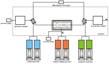
Figure 2: Schematic diagram of the experimental apparatus.

Step1. Take 4 representative core samples from the actual low-permeability rectangle reservoirs, and their basic parameters are shown in Table 1.

Step2. Get the oil mixture by mixing the kerosene and crude oil in different mass ratio, and the viscosity of the oil mixture is measured at 158˚F. Adjust the mass ratio of the kerosene and crude oil until the viscosity of the oil mixture measured at 158 ̊F is 1.4mPa.s

Step3. Adjust the compound ratio of NaCl, CaCl2 and MaCl2 until the viscosity of the salt water measured at 158˚F is 1.21mPa.s. By changing the displacement pressure gradient of oil flow to drive the core sample, the quantity of the oil flow is measured at 158 ̊F. The relationships of pressure gradient and flow were drawn, as shown in Figure 3. The displacement pressure gradient data and the corresponding quantity of the oil flow data are put into the equation (1), and the c1, c2 and c3 can be obtained, which is showed in Table 2.

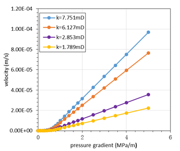
Figure 3: Non-Darcy flow curves of core simples for obtaining parameters.

E300simulation: The reservoir E300 module in Eclipse 2011 is developed for fractured heterogeneous reservoirs. E300 is used to simulate the pressure variation around a fractured vertical well in a rectangular heterogeneous reservoir. In order to meet the assumptions of equation (1), the numerical model is set as the following:

The width and the length of the rectangular heterogeneous reservoir are 1km, and there is an oil production well in the center of the reservoir, which is showed as in Figure 4a. A five-point well pattern is used to simulate the production, that is, one production well in the reservoir center and four injectors in the four corners to ensure the production of the production well. By adjusting injection volume, the oil well production under different displacement pressure can be obtained.¹³

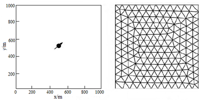
a) Reservoir well pattern     b) Meshing Schematic

Figure 4 The geometry information representation of the reservoir.

In order to describe the formation fluid heterogeneity, the triangular network of grid system is used to ensure that each crack at least has 3 grids, which is showed in Figure 4b. Therefore, the plane is divided into 20*20 meshes, and the average grid step is 50 meters. As the equation (1) describing a single-phase fluid seepage, only 1 simulation layer is divided in the vertical direction of the reservoir according to the seepage characteristics of single-phase fluid seepage. The simulation of the total number of grid 20 *20*1 = 4000.The required parameters for the numerical simulation are shown in Table 3, and the results of two methods are shown in Table 4. From Table 5, it can be seen that the relative error is under the basic control of 5%, which is in consistent with the allowable error range, suggesting that this method we offered is reliable.

Predicting water effective time

Water flooding manner are often used in China in the progress of oilfield development. After water injection, the pressure waves in the formation continue to spread from the water wells to the oil wells. When the pressure wave spread to the oil well, the oil well begins to be under the effect, and this reaching time is called Water flooding effective time.^14,15

In the secondary development of oil field in China mainland, the majority of oil fields use water flooding to improve productivity. Therefore, how to predict the water flooding response time plays an important role in adjusting the water injection pressure differential and improving efficiency of water flooding. By replacing r(t) in the equation (21) with well spacing d, and oil production q with intensity of water injection, the model can be used to predict the water flooding response time, expressed as follows.

$t=\frac{2\pi h{c}_{{}_t}}{B{J}_{{}_{ws}}(p_{{}_{inj}}-p_{{}_e})}{\left\{-\frac{C_1}{6}{r}^3-\frac{{\epsilon }_1}{({\epsilon }_2+1)({\epsilon }_2+2)}{r}^{{\epsilon }_2+2}+[\frac{C_1{r}_e}{4}+\frac{{\epsilon }_1}{2({\epsilon }_2+1)}{r}_e^{{}^{{\epsilon }_2+1}}{r}^2]\right\}|}_d^{r_e}+\frac{B\mu r_e^2{J}_{ws}(p_{inj}-p_e)}{16\pi kh}$ (48)

Much of research had been done about the water flooding effective time, and some of the specific models are as follows. Ge’s model¹⁶

$t=69.44\frac{\mu c_{{}_t}{\varphi }_0}{k}{d}^2$ (49)

Xiu’smodel¹⁷

$t=\frac{\pi c_t{\varphi }_0(\frac{dp}{dr})}{3J_{ws}(p_{inj}-p_e)}{d}^3+2.89\frac{{\mu }_w{c}_t{\varphi }_0}{k}\frac{4-e}{e}{d}^2$ (50)

Li’s model¹⁸

$t=25.128\frac{c_t{\varphi }_0(\frac{dp}{dr})}{J_{ws}(p_{inj}-p_e)}{d}^3+69.44\frac{{\mu }_w{c}_t{\varphi }_0}{k}{d}^2$ (51)

Bao Block of Bao Lang Oilfield is a low permeability reservoir,¹⁵ and the basic parameter is shown in Table 6. By using the equation (48)-(51), the effective time can be calculated. Figure 5 shows that this work has a very good match with field data, indicating that this model is effective.¹⁹

From the perspective of oil field development and production experience of China, in the process of actual oil production, the well spacing of Bao blocks is about 250meters. It is well known that from the oil practical field experience, the generally water flooding effective time is about 5 months to 9 months, and the results of the formula (48), (50) and (51) were 212.7 days, 155.2days and 173.6 days, which are consistent with the actual water flooding effective time. The calculation results of the water flooding effective time also demonstrates that the model we offered here is feasible.

Figure 6 shows that, under the condition of pressure wave spreading the same distance, the time used in the model of this paper (this work) is much smaller than Ge’s model. Because in low permeability reservoirs, our model considers the effect of starting pressure gradient and other non-linear flow factors, however, Ge’s model ignores the effect of the starting pressure gradient and reduces the flow resistance of fluid flow in the low permeability reservoir formation. So Ge’s model overestimates the flow capability of fluid in porous media. The time used in this work is a litter bigger than Li’s model and Xiu’s model. Because although the Li’s model and Xiu’s model considered the starting pressure gradient, but they mistakenly regarded the starting pressure gradient as a constant and exaggerates the flow resistance of fluid flow in the reservoir. Whenever the pressure reaches a minimum starting pressure gradient, the fluid of the formation begins to flow in the Li’s model and Xiu’s model, however, in real situations, the fluid flow in the pressure of the formation must overcome the starting pressure. So in order to reach a certain distance, it costs more time.

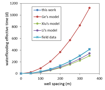
Figure 5 Effective time graph of the injection wells with different models.

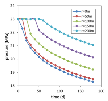
Figure 6 The map of pressure variation versus time in different locations.

Meanwhile, in the process of calculation, we found that in the model of predicting water flooding response time, the coefficient of the well spacing (That is the coefficient associated with the pilot pressure coefficient.) is much smaller than the coefficient of boundary radius (That is the coefficient associated with the starting pressure gradient.). If the water flooding response time is composed of two parts, namely, the time of associating with the pilot pressure and starting pressure gradient, the latter is much larger than the former, which indicates that in low permeability reservoirs, the effective water flooding response time is mainly associated with the starting pressure gradient. That is the reason why reducing the well spacing can effectively shorten the water flooding response time.

Sensitivity analysis

By setting the distance to the well shaft centerline, that is 0 meter, 50 meters, 100 meters, 150 meters and 200 meters, the pressure variations were observed with the time interval of 10 days. Taking different production time, which is 30 days, 60 days, 90 days, 120 days and 150 days, the distributions of pressure in the formation were observed, as shown in Figure 7.

Figure 8 shows that in the production process of the oil wells, before the pressure wave spreading to a certain location of the formation, the pressure remains at the value of the original reservoir pressure. After the pressure wave reaching the location, the pressure begins to decrease with time goes by. when spreading time is the same, in the pressure spreading range, the farther from the bottom, and the higher the pressure is.

In the process of actual oil development, many factors affect the pressure propagation speed in low permeability reservoir, such as formation properties, temperature and pressure systems. However, the model built in this paper shows that the productivity and lead pressure coefficient are the dominate factors affecting the pressure propagation speed. As the lead pressure coefficient is largely controlled by the properties of low permeability reservoirs considering actual production needs, production, permeability and viscosity are investigated in detail. By setting different oil production (that is Q=0.5 m³/d，1.0 m³/d，1.5 m³/d，2.0 m³/d), permeability (that is k=0.1mD，0.5mD，5.0mD，10mD) and viscosity (that is µ=0.5 mPa.s，3.0 mPa.s，10 mPa.s，30mPa.s), the relationships between the pressure and time are shown in Figure 7, 8 and 9. Figure 10 shows that: As the permeability of the reservoir increasing, the speed of the pressure propagation grows faster (the rate of the moving boundary increases quickly). Because with the increasing permeability, the capacity of the formation fluid flow enhances, and the corresponding reservoir resistance decreases, making the pressure wave spread easier and the moving boundary move faster.

Figure 9 shows that as the viscosity increases, the spread of the pressure wave become slowly (the rate of the moving boundary reduces). This is because that the larger the viscosity of the formation fluid is, the greater the fluid flow resistance is, and more time is needed to overcome fluid flow resistance. All of these factors make the rate of the pressure propagation becomes lower and moving boundary move slowly to the reservoir boundary.

Figure 10 shows that, under the condition of the same production time, with the oil production increasing, the faster the pressure wave propagates, and the larger the rate of the pressure wave is. Thus, for the same production time, we have to increase the rate of formation fluid flow to increase the oil productivity. Enlarging production pressure, increasing the pressure gradient as well as the rate of the pressure wave are the ways to increase the rate of formation fluid flow.²⁰ However, for the constant pressure boundary of the low permeability reservoir, there is no difference of pressure gradient in every certain location, so increasing the rate of pressure wave becomes the only way to increase oil production. On the other hand, increasing oil productivity means enlarging production differential pressure (producing pressure differential is positive with the oil production). It is necessary for the pressure wave to spread to a larger range and increase the area of pressure agitated region. All of these leads to the phenomena that with the improvement of oil well production, the pressure wave spreads faster and farther.

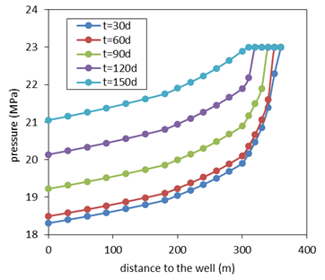
Figure 7 The formation pressure distribution at different time points.

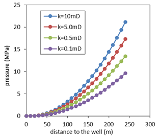
Figure 8 The influence of permeability on the spread of pressure.

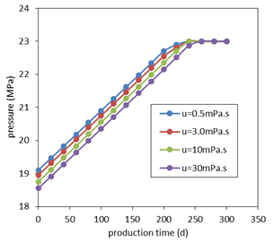
Figure 9 The influence of viscosity on the spread of pressure.

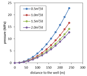
Figure 10 The influence of daily oil production on the spread of pressure.

In order to solve the defects of characterization the pressure propagation in low permeability reservoir, this paper develops mathematical models by using steady state replacement method and material balance law based on a new seepage model to study the pressure propagation phenomena in low permeability reservoirs under constant rate conditions.

For non-fracture model, in the area of pressure surge, pressure decreases with the increase of time. At the same time, within the scope of the pressure ripple, the distance from the bottom becomes farther, and the pressure becomes higher. The model of the flood-response time in the low permeability reservoir was deduced, and the relationship between the flood-response time and the injection-production well spacing is polynomial. Thus, reducing well spacing can effectively shorten the flood-response time. This model provides a theoretical basis for the water injection development and the estimation of reasonable well spacing in low permeable oil fields.

For the fracture model, a great agreement between this work and the numerical simulation results was showed in this paper, illustrating that the method in this study produces reliable transient pressure. Also, it can be seen from the sensitivity analysis that the pressure curve can be divided into four flow stream of early linear flow, mid-radial flow, late spherical flow and border control flow. The fracture scale mainly affects the early linear flow, and the fracture orientation mainly affects the late spherical flow. The method can be used to determine the optimal fracture length, fracture width and other parameters, providing theoretical guidance for reservoir engineering analysis and fracturing process design.

$p_{{}_e}$ Boundary pressure, psia

$p_{wf}$ Bottle whole pressure, psia

$p_{{}_{inj}}$ Injection well pressure, psia

$p(r)$ Pressure, psia

$q$ Oil production, MSCF/D

$r(t)$ Pressure propagation radius, feet

$r$ Radius to the center of the well axis, feet

$r_e$ Reservoir boundary radius, feet

$r_{{}_w}$ Wellbore radius, feet

$d$ Well spacing, feet

$h$ The effective thickness of the reservoir, feet

$\varphi$ Porosity, fraction

$K$ Effective permeability, mD

$\mu$ Oil viscosity, cp

${\mu }_{{}_w}$ Water viscosity, cp

$t$ Production time, h

${\rho }_{{}_o}$ Oil density, lbm/scf

$c_{{}_f}$ Liquid compressibility, psia-1

$c_{{}_l}$ Fluid compressibility, psia-1

$c_{{}_t}$ Total compressibility, psia-1

$J_{{}_{ws}}$ Solution gas-oil ratio

This article was supported by the Development of Continental Sedimentary Reservoir Simulation System " of Beijing (Grant Nos.Z121100004912001) and The Development of a New Generation of Reservoir Simulation Software of CNPC (2011A-1010).The authors would like to acknowledge support received from the RIPED, Petro China.

The author declares no conflict of interest.

1. Pascal F. Consolidation with Threshold Gradient. Inter J for Numerical and Analytical Methods in Geomechanics. 1980;5(3):547–561.
2. Yan Qinglai, He Qiuxuan, Wei Ligang. A laboratory study on percolation characteristics of single phase flow in low permeability reservoirs. Journal of Xi'An petroleum institute. 1990;5(2):1–6.
3. Huang Yanzhang . Nonlinear percolation feature in low permeability reservoir. J SOGR. 1997;4(1):9–14.
4. Yao Yuedong, Ge Jiali. Non–steady flow in low permeability reservoir. J College of petroleum engineering in the University of Petroleum. China, 2003;27(2):55–58.
5. Zhu Shengju. The propagation of pressure wave from low permeability reservoirs. J Xin Jiang petroleum geology. 2007;28(1):85–87.
6. Yang Qingli, Yang Zhengming, Wang Yifei, et al. Study on flow theory in untra–low permeability oil reservoir. J drilling and production technology. 2007;30(6):52–54.
7. Qiao Wei, Wang Liqiang, Zhang Zhigang. Pressure wave propagation of fracturing well in ultra low permeability reservoir. J XinJiang petroleum geology. 2012;33(2):196–197.
8. Liu Hailong, Wu Shuhong. The Numerical Simulation for Multi–Stage Fractured Horizontal Well in Low permeability reservoirs Based on Modified Darcy's Equation. Society of Petroleum Engineers. 2015. 17 p.
9. Wang Xiaodong. The foundation of seepage mechanics. Beijing, china, 2006. p. 11–16.
10. Shaoul J, Zelm L. Damage mechanisms in unconventional gas well stimulation–A new look at an old problem. SPE. 2011;26(4):13.
11. Boming Yu, Ping Cheng. A fractal permeability model for bi–dispersed porous media. International Journal of Heat and Mass Transfer. 2002;45(14):2983–2993.
12. Perkins TK, Kern LR. Widths of hydraulic fracture. J Pet Tecb. 1961;937–949.
13. RP Nordgren. Propagation of a vertical hydraulic fracture. J SPE. 1972;12(04):9.
14. Huang Shuangying, Chen Zhuhua, Liu Jingjun. The study of effective injection time in low permeability sandstone reservoir, taking starting pressure gradient into consider. Henan Petroleum. 2011;15(5):22–24.
15. He Ying, Xiong Chunsheng, Yang Zhengming. The study of water injection wells effective time of nonlinear flow in low permeability reservoir. Innovation and Practice seepage mechanics and engineering. 2011.
16. Ge Jiali. Oil and gas seepage mechanics Beijing. China:Petroleum Industry Press; 1982. p. 108–110.
17. Xiu Nailing, Xiong Wei, Gao Shusheng. The study of the relationship between water injection wells effective time and distance in the unstable flow of low permeability reservoir. Petroleum geology and engineering. 2008;22(1):56–57.
18. Li Yunjuan, Hu Yongle. The study of the relationship between water injection wells effective time and distance in low permeability sandstone reservoir. J Petroleum Exploration and Development. 1999;26(3):84–86.
19. Liu Rui, Jiang Hanqiao, Chen Minfeng. The classification of small complex fault block reservoirs, taking Jiangsu Oilfield for example J Xinjiang Petroleum Geology. 2009;30(6):680–682.
20. Huang Wei. Study on reasonable well pattern in horizontal well integrated development of complex small fault block. Journal of Oil and Gas Technology. 2009;3(3):105–111.