This paper revisits the popular rainfall-runoff Soil Conservation Service Curve Number (SCS-CN) methodology in perspective of Strange (1892),¹ rainfall-runoff procedure widely used in Southern parts of India. It amends the Hawkins’ (1993) concept of CN decaying with increasing rainfall (P) for complacent watersheds, which contrasts the general notion that the runoff coefficient (C) (or CN, another form of C) increases with increasing P. Its roots lie in the existing potential maximum retention (S)-CN mapping relationship. Besides suggesting a rational modification to this relationship, a more rational form of the SCS-CN methodology is presented and is found to work satisfactorily on the Strange data.

Keywords: complacent watershed, curve number, CN-P relationship, NEH-4, rainfall-runoff relation, Soil Conservation Service Curve Number method, Strange table

The Soil Conservation Service Curve Number (SCS-CN) method^2,3 is popularly used for estimation of direct runoff for a given rainfall event from small agricultural watersheds. Most of the commercial watershed models such as CREAMS,⁴ AGNPS,⁵ EPIC,⁶ and SWAT⁷ employ this methodology because of its simplicity, ease of use, lesser input data requirements, use of major runoff producing characteristics, widespread acceptance, and significant infrastructure and institutional momentum for this procedure within Natural Resource Conservation Service (NRCS).⁸

The conceptual/empirical SCS-CN model of hydrologic abstraction requires basic descriptive inputs smoothly converted into numeric values of CN⁹ reflecting the runoff potential of the watershed.¹⁰ The method takes into account the major runoff producing watershed characteristics, such as soil type, land use/ treatment, surface condition, and antecedent moisture conditions (AMCs). Since its inception, the method has been applied in several areas other than originally intended, as for example long-term hydrologic simulation,^4,11‒23 prediction of infiltration & rainfall-excess rates and hydrograph simulation,²⁴ sediment yield modeling,^25-29 partitioning of heavy metals,^30,31 determination of subsurface flow,³² urban hydrology and rainwater harvesting,^33,34 water quality,³⁵ and distributed hydrologic modeling^25,36,37 using GIS and remote sensing. For determination of subsurface flow, Yuan et al.³² modified the SCS-CN technique based on analogy derived from the plot of accumulated subsurface drainage flow against accumulated infiltration yielding subsurface drainage flow to have started after some infiltration had accumulated and the relationship to have become asymptotic to a line of 45° slope, quite similar to the popular SCS-CN rainfall-runoff relationship. The procedure was testd using the data of Little Vermilion River (LVR) watershed in East-Central Illinois.

Strange (1892)¹ studied the available rainfall and runoff in border areas of the present-day Maharashtra and Karnataka States of India and obtained runoff to rainfall ratios as functions of indicators representing catchment characteristics. These catchments were classified as Good, Average, and Bad according to their relative magnitudes of runoff coefficient. Table 1 shows the runoff coefficients (%) for different monsoon rainfall values. Here, it is presumed that the SCS-CN concept is applicable to rainfall-runoff data of any duration derived from a drainage area irrespective of its size.

As seen from Table 1, the runoff coefficient (C) (Col. 2) (ratio of direct surface runoff, Q, to rainfall, P (Col. 1)), increases with increasing P, and vice versa. Since, from SCS-CN concept.¹⁰ CN increases as C increases for a given amount of rainfall, CN should increase with P as does C. However, while describing the behavior of watersheds as complacent or standard, CN is shown to decrease with P whereas violent watersheds exhibit a decrease in CN with P up to a certain extent and afterwards, CN increases with P sharply.³⁸ To circumvent the problem, a modification is proposed to the proportional equality of the SCS-CN methodology¹⁰ and the S-CN mapping relationship. Thus, the primary objective of this paper is to resolve this issue and evaluate the proposed models using Strange data.

Existing SCS-CN methodology

The SCS-CN method is based on the water balance equation and two hypotheses expressed, respectively, as:

$P=I_a+F+Q$ (1a)

$\frac{Q}{(P-Ia)}=\frac{F}{S}$ (1b)

$Ia=\lambda S$                   (1c)

Where P, total precipitation; I_a, initial abstraction; F, cumulative infiltration excluding I_a; Q, direct runoff; and S, potential maximum retention or infiltration. The current version of the SCS-CN method assumes coefficient of initial abstraction (λ) equal to 0.2 in routine applications. λ can range from 0 to ∞.¹⁰ Combining Eqs. (4) and (5) leads to

$Q=\frac{{(P-Ia)}^2}{P-Ia+S}$ (2a)

λ = 0.2, $Q=\frac{{(P-0.2S)}^2}{P+0.8S}$        (2b)

Eq. (2) is valid for P≥I_a; Q=0 otherwise. Eq. 2a is the general form (designated as Model 1) of Eq. 2b (designated as Model 2), which is the popular form of the existing SCS-CN methodology. The only parameter S can range 0≤S≤∞, and therefore, it is mapped onto a dimensionless curve number CN, varying from 0≤CN≤100, as:

$S=\frac{25400}{CN}-254$                   (3)

Where S is in mm. CN=100 represents a condition of zero potential maximum retention (S=0), that is a completely non-abstracting impermeable watershed. On the other hand, CN=0 represents (S=∞), that is an infinitely abstracting watershed. Mishra and Singh¹⁰ described CN as an index of runoff potential of a watershed corresponding to 10 inches (=254mm) of rainfall. This logic is also supported by the fact that routine RS-GIS applications frequently distinguish two watersheds in terms of CN for their runoff-producing (or hydrologic) potential, ignoring the fact that CN also depends on rainfall. Thus, it is more rational to describe the runoff producing potential of a watershed for a particular rainfall amount.

S can be determined from Eq. 2b as:

$S=5(P+2Q-\sqrt{(Q(4Q+5P)})$ (4)

Notably, the SCS-CN method excludes the effect of slope on runoff yield and, in turn, on the resulting CN.

Significance of l

l (Eq. 1c) actually represents the ratio of initial abstraction (I_a) to parameter S. Since I_a included climate-dependent evaporation, soil-dependent initial infiltration, surface feature (land use)-dependent surface detention, and vegetal (land cover) interception, and all these affect the surface runoff potential described by CN (or S), and therefore, it is not out of order to describe it as a function (or fraction or multiple) of S (or CN). S, in turn, is mapped on to CN, and therefore, it is not out of order to foresee the dependency of l on CN (or C) that varies with P.³⁸ Because of larger variability, I_a=0.2S relationship has been the focus of discussion in literature and modification since its inception. Aron et al.³⁹ suggested l≤0.1 and Golding⁴⁰ provided l values for urban watersheds depending on CN as l=0.075 for CN≤70, l=0.1 for 70<CN≤80, and l=0.15 for 80<CN≤90. Ponce & Hawkins⁴¹ suggested that the fixing of l as 0.2 might not be the most appropriate number, and that it should be interpreted as a regional parameter. Hawkins et al.⁴² found that a value of l=0.05 fitted the data better and therefore was more appropriate for use in runoff calculations.

Mishra & Singh⁴³ suggested that λ can take any non-negative value. Mishra & Singh²⁴ developed criterion for the applicability of SCS-CN method based on runoff coefficient (C) and l variation. They defined the applicability bounds for the SCS-CN method as for l≤0.3, I_a/P≤0.35 and C≥0.23. Since P relies on climate/meteorological characteristics of the region, Jain et al.¹⁷ proposed a more general non-linear I_a-S-P relation, and Mishra et al.⁴⁴ used I_a-S-M relationship based on the hypothesis that I_a largely depends on the initial soil moisture (M). Thus, there exists a sufficient scope for improvement.

Significance of CN

Mishra and Singh¹⁰ described the significance of CN as a degree of saturation (S_r) of an initially completely dry watershed due to 254mm (=10inches) of rainfall. For I_a=0, Eq. 1a can be recast as,

$100\frac{F}{S}=C{N}_P=\frac{100}{1+S/P}$                     (5)

Which describes the P-dependent CN_P for a given S. For P=254mm (=10inches), CN_p=CN as described by Eq. 3. It is worth noting that the direct use of CN in the proportionality hypothesis (Eq. 1b) for computing Q is restricted, because CN, by definition, corresponds to the 254mm base rainfall amount, not to the actual amount. Therefore, Eq. 2 with I_a=0 should be resorted to computation of Q for a given rainfall amount.

In terms of CN, the runoff factor C (=Q/P) can be defined from Eq. 2 (for I_a=0) as:

$C=\frac{1}{1+\frac{254}{P}\left(\frac{100}{CN}-1\right)}$         (6)

Figure 1 depicting the variation of C with CN and P shows that for a given P, as C increases, CN also increases; for a given C, CN increases with decreasing P; and for a given CN, C increases as P increases. The first condition is realizable when the watershed characteristics change, as for example, from agriculture to urban or vice versa. The last condition of a given CN, implying a particular type of watershed with certain wetness or of specific runoff potential, is realizable as C increases with P, as shown by Strange data described later. However, the second condition is hard to realize for the reason that C is forced to remain constant with changing P, which it actually can’t, and therefore, CN (which is a constant) is forced to exhibit a decreasing trend with increasing P for enabling C to remain at a fixed value in Eq. 6. Such behaviour can also be explained as follows.

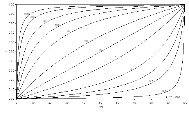
Figure 1 Variation of runoff factor (C) with curve number (CN) and precipitation (P, inch). 1inch=25.4mm.

Re-writing Eq. 4 in terms of C and P, it can be shown that S (or S_P) is a function of both C and P. C increases with P¹ and S (or S_P) is directly proportional to P (Eq. 4). Thus, S (or S_P) will increase with increasing P, and vice versa, and, from Eq. 3, CN is inversely related to S (or S_P). It leads to the inference that CN is inversely related to P. Such unrealistic behaviour has led to several misunderstandings/misinterpretations. To circumvent the problem, a modification is needed in the SCS-CN application procedure, as follows. From given P-Q data, compute S_P from Eq. 4, and CN_P from Eq. 5. Here, subscript ‘P’ to S or CN refers to their correspondence with P. Similarly, CN corresponding to 254mm of P can be defined as CN₁₀ or simply CN from Eq. 3. Since it represents the runoff potential of a watershed for a fixed amount of rainfall, it is a better indicator to predict the comparative effect of watershed characteristics.

Following Hawkins,³⁸ Strange data (Table 1) is plotted in Figure 2. In this figure, solid lines show the variation of CN (derived from Eqs. 4 and 3) with P for varying C (=Q/P) values. As seen, for any fixed C-value, CN decreases with P, as described above. The dotted lines correspond to three watersheds described by Strange as Good, Average, and bad watersheds depending on their runoff generating potential. A Good watershed exhibits a high and Bad a low runoff generating potential, and Average falls in between. Thus, consistent with the literature, let the Bad watershed be described as Complacent, Average as Standard, and Good as violent watershed. Notably, for a watershed to be violent, CN should increase rapidly with increasing P.

Figure 2 Plot of Strange data in the existing CN perspective.

As seen from Figure 2, the complacent type behaviour of the watershed closely follows the line C=0. C can however be equal to 0 under three situations: (a) P£0.2S, (b) P=0, and (c) S=¥. Here, the second situation is clearly improbable for an event to occur (as P is non-negative) whereas the first and last ones are most likely to prevail. Thus, for C=0, P has always to be less than 0.2S, and therefore, has to follow C=0 line. In other words, complacent behaviour is realizable only if it is an absolutely zero runoff potential watershed, an idealized situation. On the other hand, CN values are seen in the same figure to range (12.63, 68.23). Similarly, the data of the standard watershed exhibits C to vary from 0.001 to 0.45 and CN values range (16.63, 68.23). The data of Good, Average, and Bad watersheds exhibit C to vary in the range (0.001, 0.6), (0.001, 0.45), and (0.001, 0.3), respectively. Up to the reasonably high rainfall of 254mm (=10inches), C-values range (0.001, 0.043), (0.001, 0.032), and (0.001, 0.021), respectively, indicating all watersheds to be low runoff producing watersheds.

Following the present understanding on the existing S-CN relationship (Eq. 3), the behaviour of the complacent watersheds can be described as follows. All three watersheds closely follow C=0 line until P exceeds I_a. It will exist under all circumstances in nature as the direct surface runoff always starts with zero, and therefore, every watershed has to follow it and, in turn, has to be complacent in nature. When P exceeds I_a, the behaviour of watershed is actually reflected by the increase in both P and P-dependent C, rather than CN (which is for P=254mm). The gradual and abrupt rate of rise in C leads to the description of watersheds as standard and violent, respectively. At what P-magnitude, this rise will be experienced in a watershed will depend on watershed characteristics affecting the runoff generating potential.

Figure 3 shows CN-P and CN_P-P relations to describe the behaviour of three types of watersheds described by Strange. As seen, CN_P exhibits a more rational behaviour than does CN with increasing P for all three datasets; as P increases, CN_P also increases and C (not shown) also increases, consistent with the above notion.

Figure 3 CN and CN_P versus P relations for strange datasets. Note: Strange data best fitted with CN using 2 period moving averages.

The methodology proposed (designated as Model 3 for CN and Model 4 for CN_p) can be described in steps as follows:

1. Determine S or S_P from Eq. 4 using the observed P-Q dataset for a watershed.
2. Determine CN from Eq. 3 and CN_P from Eq. 5.
3. Develop a relationship between CN or CN_P and P for the watershed.
4. For known P, derive CN or CN_P from the respective relation for field application.

Application of these models is demonstrated using Strange (1892) data.

Modification to the formulation of SCS-CN methodology

The basic formulation of SCS-CN methodology is modified keeping in view the decreasing trend of CN with P in Figure 3. To this end, the proportional equality hypothesis is re-written and revised as follows:

$\frac{F(P-I_a)}{Q}=S=S_o{e}^{-\alpha P}$                                      (7)

Where S_o is the initial storage space (or potential maximum retention when P=0) (mm) and α is a decay coefficient (mm^-1). The right hand side of Eq. 7 is consistent with the work of Mishra and Singh,¹⁰ the storage space actually decreases as rainfall grows with time. Taking I_a=0, Eq. 7 can be reformulated as:

$Q=\frac{P^2}{P+S_o{e}^{-\alpha P}}$                                    (8)

Which is the revised model formulation. From Eq. 8,

$\frac{S_o}{P}=\frac{1-C}{C{e}^{-\alpha P}}$                         (9)

Following Eq. 5, revised CN can be described as follows:

$C{N}_o=\frac{100}{1+S_o/P}=\frac{100C{e}^{-\alpha P}}{1+(e^{-\alpha P}-1)C}$    (10)

For CN_o≥0, C≥0 and/or P£¥, which is justifiable. For CN_o£100, C£1, which is again reasonable. However, Eq. 10 shows CN to decrease with P, but for constant C, a physically unrealizable condition. When C=0, CN_o=0 and when C=1, CN_o=100. In addition, α=0 in Eq. 8 implies that S_o does not vary with precipitation (or time),¹⁰ which contrasts the fundamental decay behaviour of infiltration with time. Thus, Eq. 8 presents a more realistic formulation than the existing one. It is designated as Model 5 in the forthcoming text.

Model 5 (Eq. 8) can be further (coarsely) approximated to

$Q=\frac{P^2}{P+S_o(1-\alpha P)}$                                                                                                                   (11)

Or                                       $Q=\frac{P^2}{(1-\alpha S_o)P+S_o}=\frac{P^2}{aP+S_o}$                (12)            

Where a=1– αS_o. Eq. 12 is the Modified SCS-CN model proposed by Mishra and Singh (1999). From Eq. 12,

$\frac{S_o}{P}=\frac{1-C}{(1-\alpha P)C}$                                                                   (13)

As C®0, S_o/P® ¥, and as C®1, S_o/P® 0. From Eq. 5,

$CN=\frac{100(1-\alpha P)C}{1-\alpha PC}$                (14)

As C®0, CN®0, and as C®1, CN®100, consistent with the general notion that CN increases with C, and vice versa. Similar to Model 5, CN can be shown to decrease with P, but for constant C, a physically unrealizable condition. Furthermore, for CN to be non negative (the applicability criterion),

$\alpha PC=\alpha Q\le 1 and \alpha P\le 1$              (15)

Eq. 11 or Eq. 12 is designated as Model 6 in the forthcoming text.

As above, Strange described the watersheds as Good, Average, and Bad according to their relative magnitudes of yield or runoff. It is again worth emphasizing here that the Strange monsoon season data (Table 1) was used considering that the SCS-CN concept is applicable to any duration (including seasonal) rainfalls. The correlation equations of best fitting lines relating percentage C are expressed as Strange (1892):

For Good catchment:

$ForP<250mm, C\left(\%\right)=7\times {10}^{-5}{P}^2–0.0003P,R^2=0.9994$ (16a) 

$For250<P<760mm, C\left(\%\right)=0.0438P–7.1671,R^2=0.9997$ (16b)

$For250<P<760mm, C\left(\%\right)=0.0438P–7.1671,R^2=0.9997$ (16c)

For Average catchment:

$ForP<250mm, C\left(\%\right)=6\times {10}^{-5}{P}^2–0.0022P+0.1183,R^2=0.9989$ (17a)

$For250<P<760mm, C\left(\%\right)=0.0328P–5.3933,R^2=0.9997$ (17b)

$For760<P<1500mm, C\left(\%\right)=0.0333P–5.7101,R^2=0.9999$ (17c)

For Bad catchment:

$ForP<250mm, C\left(\%\right)=4\times {10}^{-5}{P}^2–0.0011P+0.0567,R^2\text{= }0.9994$  (18a)

$For250<P<760mm, C\left(\%\right)=0.0219P–3.5918,R^2=0.9997$  (18b)

$For760<P<1500mm, C\left(\%\right)=0.0221P–3.771,R^2=1.0$  (18c)

Where C(%) is percentage; runoff coefficient, ratio of seasonal runoff to seasonal rainfall in percent (non-dimensional), P, monsoon season rainfall in mm, and R², coefficient of determination.

Since there is no appreciable runoff due to rains in dry (non-monsoon) period, the monsoon season runoff volume has been taken as annual yield of the catchment.¹ This table can be used to estimate the monthly yields also in the monsoon season. It is however to be used with the understanding that the table relates cumulative monthly rainfall since the beginning of the season and the corresponding cumulative runoff.

Considering the above Strange data as observed, the use of both CN and CN_P concepts is shown to describe this data in Figure 3. As seen, CN first decreases with increase in P and then after a certain extent (i.e. P=254mm =10inches), CN increases with increasing P. Thus, the same CN-concept shows two different types of behaviour with increasing P. It is resolved by plotting CN_P against P (Figure 3). This data has been used for performance evaluation of 6models described above and summarized in Table 2.

The model application results are shown in Table 3 and Figures 4A-4C. As seen, Model 1 is the generalized form of the existing SCS-CN model, i.e. Model 2. CN for both the models is derived from Eq. 3. Both Models 3 & 4 are based on Eq. 2b and Eq. 4. The former employs Eq. 3 for CN determination whereas the latter one employs Eq. 5 for CNp determination. CN- and CNp-values for these models are derived from the following relations (Figure 3):

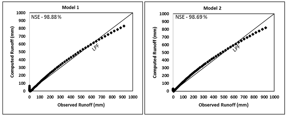
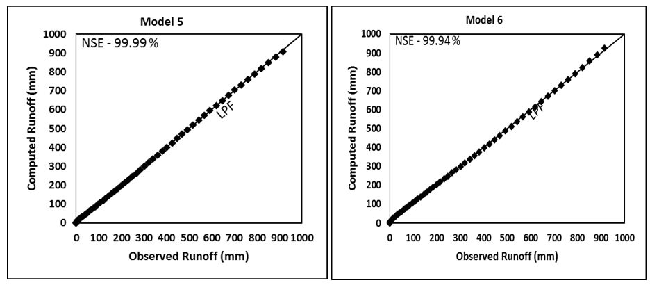
Figure 4A Evaluation of Models 1-6 by comparing the computed runoff (mm) with the observed runoff (mm) of Good watershed (Strange, 1892). LPF represents the line of perfect fit. NSE, Nash and Sutcliffe Efficiency.

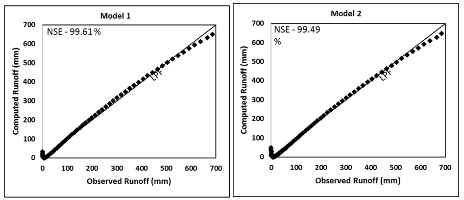
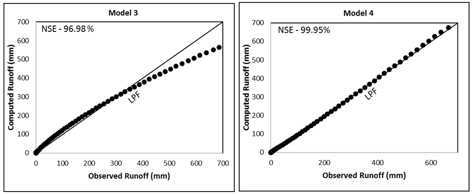
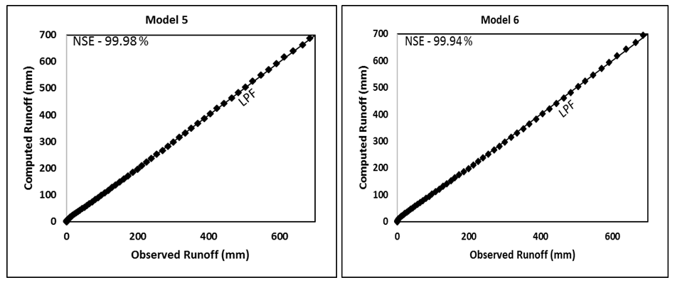
Figure 4B Evaluation of Models 1-6 by comparing the computed runoff (mm) with the observed runoff (mm) of Average watershed (Strange, 1892). LPF represents the line of perfect fit. NSE, Nash and Sutcliffe Efficiency.

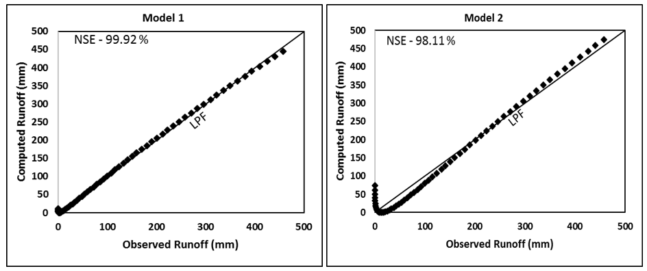
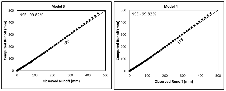
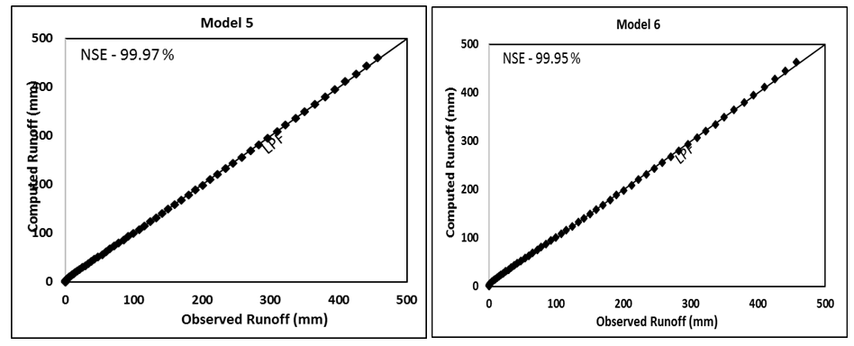
Figure 4C Evaluation of Models 1-6 by comparing the computed runoff (mm) with the observed runoff (mm) of Bad watershed (Strange, 1892). LPF represents the line of perfect fit. NSE, Nash and Sutcliffe Efficiency.

For Model 3,

CN=3E-06P-0.0571P+43.225           (for Good watershed)                                                          (19a)

CN=134.89P^-0.301                                  (for Average watershed)                                     (19b)

CN=227.29P^-0.413                                  (for Bad watershed)                                                            (19c)

These CN relations can be further improved/simplified significantly by using CN_P in place of CN (for Model 4),

CNp=0.0343P+16.435                       (for Good watershed)                                                          (20a)

CNp=0.0267P+17.06                          (for Average watershed)                                     (20b)

CNp=0.0192P+17.491                       (for Bad watershed)                                                            (20c)

In Eqs. 10 & 14, 0£CN or CNp£100. Model 5 is based on Eq. 8, and Model 6 on Eq. 11. The former is the general form of the latter. CN_o for both these models is derived from Eq. 3 so as to bring all CN-values at one P (=254mm = 10inch)-scale.

As seen from Table 3, Good watershed has the highest runoff coefficient (C) (derived from mean values of rainfall and runoff), Bad the lowest, and Average in between these two. Such order of runoff generating potential is described by CN (or CN_o) values derived (for the same P=254mm) from all model applications. All the models generally performed extremely well on all watersheds. Model 3 performed the poorest. l of Model 1 is seen to have ranged from 0.07 (for Bad watershed) to 0.29 (for Good watershed). Thus, l appears to be mean C (or CN)-dependent. It is of paramount importance in field applications as a proper prescription of average C-dependent l-value can enhance the results significantly. l®0 appears to be reasonable for Bad type of watersheds, largely for the reason that such watersheds exhibit very high S (or low CN) value to describe a certain value of initial abstraction (I_a=lS). Similarly, a relatively high l-value is proper for Good type of watersheds as these watersheds exhibit very low S (or very high CN) values. Bias in Table 3 is presented to indicate whether a model over (positive)- or under (negative)-predicted the runoff.

The application results of Models 3 and 4 indicate that the latter is in general an improvement over the former one and, therefore, assert that the pre-derived CNp-P relationship for a watershed can be an improved alternative for runoff predictions using Model 2. In addition, as shown in Figure 5, the use of Eq. 5 better describes the Good, Average, and Bad watersheds just based on CNp or C-values.

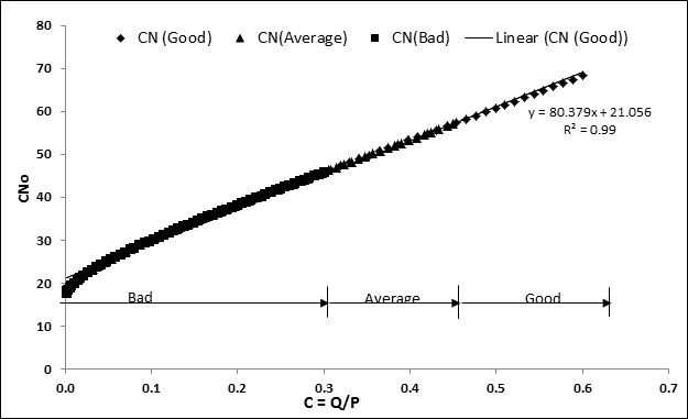
Figure 5 C-CNp relationship (Model-4 consisting of Eqs. 2b, 4, and 6) for description of watershed behaviour.

Model 5 is a general form of Model 6, and it is also exhibited by their application results. Both the parameters α and S_o, respectively, exhibit consistently decreasing and increasing trends with Good to Average and to Bad watersheds. In addition, Eq. 8 of Model 5 when plotted for a specific value of α, the resulting C-CN_o (Figure 6) and CN_o-P (Figure 7) relations more rationally describe the behavior of the three types of watersheds.

Figure 6 C-CN_o relationship for Model 5 (α=0.0001).

Figure 7 Variation of CN with P (mm) for three types of watersheds for Model 5 with α=0.0001.

Thus, in order of preference all the models can be preferred for generally all watersheds. Among these, Model 3 is the least preferable. For improved applications, mean C-l can be prescribed for a watershed. Model 4 can be preferred if CNp-P relations are established. Model 6 along with mean C-α relation can also be a substitute for all watersheds.

The following can be derived from the present study:

1. The description of three Good, Average, and Bad watersheds based on decreasing CN trend with increasing P is physically not justifiable as it contrasts the increasing trend of C (or CN) with increasing P.
2. The proposed CNp-P relation (Eq. 5) describes more rationally the behaviour of the above three watersheds.
3. The proposed modification to the application approach of the popular SCS-CN methodology (i.e. Model 4) is more rational, as it describes consistent C-CN-P behavior, and has the efficacy to describe the watershed behavior more scientifically and resolve the issue of CN decaying with increasing rainfall (P).
4. The proposed Models 5 & 6 have the power to physically describe the behavior of three watersheds and are equally suitable for these watersheds.
5. Model 1 and Model 2 performed extremely well for all the watersheds. However, the prescription of mean C-l (Model 1) and/or CNp-P (Model 4) relationships for a watershed can improve the application results significantly.^45‒47

None.

The authors declare that there is no conflict of interest.

None.

1. Subramanya K. Engineering Hydrology. Fourth Edition, McGraw Hill Edu. (India) Pvt Ltd, New Delhi. 2013a. p. 534.
2. SCS. National Engineering Handbook, Hydrology. Section 4, Soil Conservation Service, US Department of Agriculture, Washington DC. 1956.
3. SCS. Hydrology National Engineering Handbook. Supplement A, Section 4, Chapter 10, Soil Conservation Service, USDA, Washington, DC. 1972.
4. Knisel WG. CREAMS: a field–scale model for chemical, runoff and erosion from agricultural management systems. Conservation Research Report No. 26, South East Area, US Dept. of Ag., Washington, DC. 1980.
5. Young RA, Onstad CA, Bosch DD, et al. AGNPS: a nonpoint–source pollution model for evaluating agricultural watersheds. J Soil & Water Conservation. 1989;44(2):168–173.
6. Sharpley AN, Williams JR. EPIC—Erosion/Productivity Impact Calculator: 1. Model Documentation. US Department of Agriculture Technical Bulletin No. 1768. US Government Printing Office, Washington, DC. 1990.
7. Arnold JG, Williams JR, Srinivasan R, et al. SWAT: Soil and Water Assessment Tool. USDA–ARS, Grassland, Soil and Water Res. Lab, Temple, TX. 1996.
8. Garen D, Moore DS. Curve number hydrology in water quality modeling: use, abuse, and future directions. J Am Water Resour Assoc. 2005;41(2):377–388.
9. Bonta JV. Determination of watershed curve number using derived distributions. J Irrig & Drain Engg. 1977;123(1):234–238.
10. Mishra SK, Singh VP. Soil Conservation Service Curve Number (SCS–CN) Methodology. Kluwer Academic Publishers, Dordrecht. 2003.
11. Williams JR, La Seur V. Water yield model using SCS curve numbers. J Hydraulic Engg. 1976;102(9):1241–1253.
12. Hawkins RH. Runoff curve number with varying site moisture. J Irrig and Drain Engg. 1978;104(4):389–398.
13. Woodward DE, Gbuerek WJ. Progress report ARS/SCS curve number work group. Proceedings of ASCE Water Forum. ASCE, New York. 1992;378–382.
14. Pandit A, Gopalakrishnan G. Estimation of annual storm runoff coefficients by continuous simulation. J Irrig and Drain Engg. 1996;122(4):211–220.
15. Mishra SK, Singh VP. Long–term hydrological simulation based on soil conservation service curve number. Hydrol Process. 2004a;18(7):1291–1313.
16. Jain MK, Mishra SK, Babu S, et al. Enhanced runoff curve number model incorporating storm duration and a nonlinear Ia–S relation. J Hydrol Engg. 2006b;11(6):631–635.
17. Jain MK, Mishra SK, Babu S, et al. On the Ia–S relation of the SCS–CN method. Nord Hydrol. 2006a;37(3):261–275.
18. Sahu RK, Mishra SK, Eldho TI, et al. An advanced soil moisture accounting procedure for SCS curve number method. Hydrol Process. 2007;21(21):2827–2881.
19. Kannan N, Santhi C, Williams JR, et al. Development of a continuous soil moisture accounting procedure for curve number methodology and its behavior with different evapotranspiration methods. Hydrol Process. 2008a;22(13):2114–2121.
20. Durbude DG, Jain MK, Mishra SK. Long–term hydrologic simulation using SCS–CN based improved soil moisture accounting procedure. Hydrol Process. 2011;25(4):561–579.
21. Sahu RK, Mishra SK, Eldho TI. An improved AMC–coupled runoff curve number model. Hydrol Process. 2010;24(10):2834–2839.
22. Babu PS, Mishra SK. Improved SCS–CN–Inspired Model. J Hydrol Engg. 2012;17(11):1164–1172.
23. Jain MK, Durbude DG, Mishra SK. Improved CN–Based Long–Term Hydrologic Simulation Model. J Hydrol Engg. 2012;17(11):1204–1220.
24. Mishra SK, Singh VP. Validity and extension of the SCS–CN method for computing infiltration and rainfall–excess rates. Hydrol Process. 2004b;18(17):3323–3345.
25. Mishra SK, Singh VP. Soil conservation service curve number (SCS–CN) methodology. Kluwer, Dordrecht, The Netherlands. 2003a.
26. Mishra SK, Tyagi JV, Singh VP, et al. SCS–CN based modeling of sediment yield. J Hydrol. 2006b;324(1-2):301–322.
27. Tyagi JV, Mishra SK, Singh R, et al. SCS–CN based time distributed sediment yield model. J Hydrol. 2008a;352(3-4):388–403.
28. Singh PK, Bhunya PK, Mishra SK, et al. A sediment graph model based on SCS–CN method. J Hydrol. 2008;349(1-2):244–255.
29. Bhunya PK, Jain SK, Singh PK, et al. A simple conceptual model of sediment yield. Water Resour Manage. 2010;24(8):1697–1716.
30. Mishra SK, Sansalone JJ, Singh VP. Partitioning analog for metal elements in urban rainfall–runoff overland flow using the soil conservation service curve number concept. J Env Engg. 2004b;130(2):145–154.
31. Mishra SK, Sansalone JJ, Glenn DW, et al. PCN based metal partitioning in urban snow melt, rainfall/runoff, and river flow systems. J Am Water Resour Assoc. 2004c;40(5):1315–1337.
32. Yuan Y, Mitchell JK, Hirschi MC, et al. Modified SCS Curve Number Method for predicting sub surface drainage flow. Trans ASAE. 2001;44(6):1673–1682.
33. Kadam AK, Kale SS, Pande NN, et al. Identifying potential rainwater harvesting sites of a semi–arid, basaltic region of western India, using SCS–CN method. Water Resour Manage. 2012;26(9):2537–2554.
34. Singh PK, Yaduwanshi BK, Patel S, et al. SCS–CN based quantification of potential of rooftop catchments and computation of ASRC for rainwater harvesting. Water Resour Manage. 2013;27(7):2001–2012.
35. Ojha CSP. Simulating turbidity removal at a river bank filtration site in India using SCS–CN approach. J Hydrol Engg. 2012;17(11):1240–1244.
36. White D. Grid–based application of runoff curve numbers. J Water Resour Planning and Manage. 1988;114(6):601–612.
37. Moglen GE. Effect of orientation of spatially distributed curve number in runoff calculations. J Am Water Resour Assoc. 2000;36(6):1391–1400.
38. Hawkins RH. Asymptotic determination of runoff curve numbers from data. J Irrig and Drain Engg. 1993;119(2):334–345.
39. Aron G, Miller AC, Lakatos DF. Infiltration formula based on SCS curve numbers. J Irrig and Drain Div ASCE. 1977;103(4):419–427.
40. Golding BL. Discussion of runoff curve numbers with varying soil moisture. J Irrig Drain Div ASCE. 1979;105(IR4):441–442.
41. Ponce VM, Hawkins RH. Runoff curve number: Has it reached maturity? J Hydrol Engg. 1996;1(1):11–19.
42. Hawkins RH, Woodward DE, Jiang R. Investigation of the runoff curve number abstraction ratio. Pap presented at USDA–NRCS Hydraulic Engineering Workshop, Tucson, Arizona. 2001.
43. Mishra SK, Singh VP. Another look at the SCS–CN method. J Hydrol Engg. 1999;4(3):257–264.
44. Mishra SK, Sahu RK, Eldho TI, et al. An improved Ia–S relation incorporating antecedent moisture in SCS–CN methodology. Water Resour Manage. 2006a;20(5):643–660.
45. Michel C, Vazken A, Charles P. Soil conservation service curve number method: how to mend among soil moisture accounting procedure? Water Resour Res. 2005;41(2):1–6.
46. Mishra SK, Singh VP. A re–look at NEH–4 curve number data and antecedent moisture condition criteria. Hydrol Process. 2006;20(13):2755–2768.
47. Mishra SK, Singh VP. SCS–CN method: Part–II: Analytical treatment. Acta Geophysica Polonica. 2003b;51(1):107–123.