We propose an exponential type growth model over time for yield of a tuber crop turmeric observed in a growth experiment, the model is motivated from elementary consideration of proportionate growth. The experiment was conducted to see the effect of seed weight on yield and continued over a period of two seasons to ensure adequate color and high yield of turmeric. Turmeric plants sprouted for a second time in same pits for second season after a dormant period, as the crop was not harvested at the end of first season for a higher production. It is thus of interest to obtain growth curve of yield over time in order to understand the underground growth process over extended time period. The growth model is partly based on initial seed weight, plant height and maximum length of leaves. Farmers usually express gain in yield as a multiple of seed weight. Information on multiplicative factor of seed weight to crop yield is incorporated in the model. Apart from seed weight, maximum of plant height over time is seen to be a good predictor for yield. Exponential growth model is supplemented by additional auxiliary variables via nonparametric regression. An exponential type growth curve may be appropriate for yield data only for a bounded time region.

Overall growth curve for yield of all the plants may be attributed to the mean seed weight; the growth curve from mean seed weight is close to overall response curve. Observations on plant height and maximum leaf length in the plants over time in the conducted experiment are available only for the first season due to resource constrains. Yield data for different seed weights are available only at the end of second season; this keeps the experimental set up undisturbed throughout the experiment. Estimation of yield over time under such a restricted setup is significant and useful for adequate planning for high yield. Seed weight 10 g of turmeric is seen to produce best proportionate yield to the tune of 8.71 times in lateritic alluvial soil of Giridih, Jharkhand (India) at the end of second season. Proliferation rates of the growth curves are obtained. A characterization of the discrete version of exponential growth curve over unequal spacing is proved.

Keywords: exponential growth, lowess regression, principal component, proliferation rate

Turmeric is a tuber crop with many medicinal values. This is extensively used in culinary of different countries as useful spice. With powerful health promoting properties e.g., see Holt et al.,¹ this is under extensive medical research. India is the largest producer of turmeric. Growth experiments with seed weights 10g, 15g, 20g, 25g and 30g are conducted in an experimental plot of Giridih farm of Indian Statistical Institute during the years 2014–2016. The problem is to study the growth curve of yield over time and to identify the appropriate seed weight and the best linear predictor of yield based on observable above ground auxiliary variables in usual or log–log scale over extended period of time for two seasons to achieve a high yield. The Latin Square Design (LSD) and numbering of the plants used in the growth experiment is similar to that stated in Dasgupta,² without giving any consideration to the skin texture of seed corms at the present study. 5X5 LSD is shown below.

A B C D E

B C D E A

C D E A B

D E A B C

E A B C D

In the field experiment the characteristic of the planted turmeric seed of yam corm tested are represented by Latin letters; i.e., A: 10; B: 15; C: 20; D: 25; E: 30 are weights in grams of the seed. The above Latin square were repeated 4 times side by side in a block of two squares, and the pit–holes are numbered 1 to 5 for the first row in reverse direction i.e., as E; D; C; B; A; in the first experiment. The numbering goes on in the same row of adjacent second design as 6 to 10, and so on. Finally, the pit holes are numbered 91 to 95 for the last row of the 2X2 block viz., D; C; B; A; E; in the third experiment; and the numbering goes on in the same row i.e., the 10^th row with above combination of alphabets layout in adjacent design number 4, as 96 to 100. This completes the layout of 100 pits in experiment 1.

Adjacent to this, another such experiment with 100 pits of similar layout is simultaneously undertaken as experiment 2. Thus the total number of pits is 200 in the turmeric growth experiment conducted in Giridih farm during 2014–2016. A little organic manure like vermicompost was administered at the beginning of the experiment. All the seed corms germinated to turmeric plants. For eight plants the yield is nil, and for two plants the initial weight equaled to the final weight. Therefore we concentrate on the remaining 190 turmeric plants in data analysis; see (Table 1) (Table 2). Above ground auxiliary variables on biomass like maximum leaf length and plant height are available only for the first season due to resource constrains. There is a time gap of about three and half months that can be considered rest time for seed corm growth in the interim period. This is the time in between two seasons when the turmeric corm remained dormant underground.

Yield data of the first season is unavailable, as the weights were not recorded by taking the yield out of the ground at the end of that season, thus the experimental set up remained undisturbed. To ensure adequate weight and color of the crop, turmeric in Giridih farm is harvested at the end of second season. This is a standard practice farmers often take recourse to in anticipation of a good harvest over extended period of cultivation. In section 2 we search for a growth mode. Maximum plant height is seen to be a good predictor of the yield and this variable is used to calibrate the exponential growth model via nonparametric regression of lowess and spline smoothing.

The proposed procedure blends the information from observable auxiliary variables with yield data obtained at the end of second season. A modification of exponential growth curve is looked into for modeling the data; the exponential part involving time in it plays the dominant role. Further, for seed weight 10g, auxiliary information from both seasons is utilized to draw the growth curve of turmeric over the entire time period. Proliferation rate of these growth curves exhibit inherent features of the model. Seed weight 10g of turmeric is superior for high yield at the end of second season. Observations on auxiliary variables viz., plant heights and leaf lengths are taken on unequal time intervals. A discrete version of the growth model with unequal spacing of time is characterized in section 3. Results are discussed in section 4.

The yield data is unavailable at the end of first season; we have to interpolate it for this interim period. Sometimes crop produced in a season is reported in terms of multiple of seed weight planted i.e., as the ratio of yield to initial weight. Under the assumption of proportionate increase of k≥1 times the seed weight, the yield y=y (t) from seed weight w is kw after first season, and k²w at the end of second season. An estimate of k²=k² (w) being available from yield data of second year; seed specific growth may be ascertained i.e., log(y/w)=at; where k=exp(a), a=1,2 Preliminary estimates of k for different seed weights from recent data indicate that these estimates in the same plot of land do not vary too much. The model can be tuned, if plant lifetime, calculated as the difference (in days) of sprouting of a plant in the first season till the end of the plant survival up to the second season, is incorporated in a plant specific model instead of a broad classification of season. The available information on plant height (x₁) and maximum length of leaves (x₂) may also be incorporated for model accuracy. After attempting several closed form of expressions involving linear, quadratic, logarithmic function etc. of the variables involved, for an appropriate t in regression, with seed weight w appearing as divisor of variables for scaling; the following candidate model provided a value of multiple regression square, R²=0.2121 out of 190 observations with a₀=24.42646; a₁=0.05301; b₁=1.27693; b₂=0.09871;

log(y/w)=a₀+a₁t+b₁ log(X₁/w)+b₂ log x₂/w ... (1)

Where we considered maximum over plant lifetime on x₁ and x₂ in individual plants, for we considered the plant lifetime in place of t in the model. The variables plant height and leaf length is time dependent. Inclusion of these in the model improves the value of R². The variables lifetime and plant height are significant in analysis of variance. We recheck the model by fixing the lifetime t at 610 and 611 days. Many plants are available at those lifetimes in observed data. Considering the plants with assigned lifetime, the number of such plants are 42 in each category. The value of R² in these fixed profile of (1) with the following model are 0.3187 and 0.2266 respectively.

log (y/w)=a₀+b₁ log(x₁/w)+b₂ log(x₂/w) ... (2)

When the dormant time period [16.3.15, 30.6.15] of 107 days i.e., the time of rest of underground corm in between two seasons is deleted from the total lifetime of the plants i.e., t is replaced by (t–107), the regression equation remains the same with a change in the value of constant; the new value being a₀=18 a₀ 75488. Exponential growth is usually observed in the beginning of a growth process when resources are unlimited, an example is bacterial growth, see e.g., Slavov et al.³ for exponential growth of cells at constant rate while remodeling some cell properties. However, this may not be the case of turmeric experiment and we may take the growth pattern of related variables like plant height and maximum leaf height into account to compute the yield growth curve. To this end we compute the first principal component 0.9844981x₁+0.1753952x₂ (and the eigen values 130.94762, 73.15037) that explains maximum variation of data consisting of the variables x₁ and x₂ in all plants in the first season.

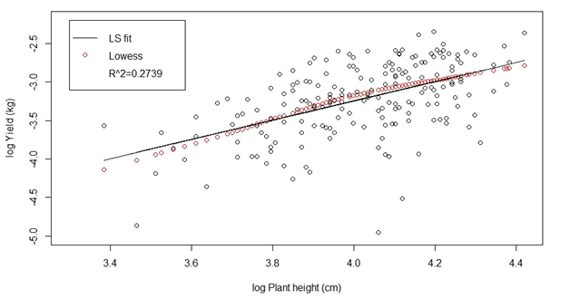
The coefficient of the first variable is near 1. The first variable being dominant we may consider the growth curve of plant height to calibrate the exponential growth model. In modified exponential growth we consider the maximum lifetime of plants with relevant seed weight to compute the parameters of exponential model, and then we compute the weighted average slopes of exponential growth and plant height growth and draw the curve starting from the seed weight 20 g at time zero maintaining the weighted average slope over different time point. The weights (p; 1–p) are so selected as to maintain the rate of growth of the auxiliary variable and that for exponential modeled yield at the same scale; p=10^–4 for seed weight 20g. This scaling is suggested from the slope of regression line of yield on plant height. Regulated by inherent related processes in the plants, the growth rates are different for plant height and for turmeric deposition underground. The slope of (Figure 1) confirms the choice of p; as seen from the slope of regression of yield on plant height. The same choice also works for other seed weights. Figure 2 shows the residuals are symmetric. The value of R² has slightly improved in log–log scale of variables, and the resultant residuals are asymmetric as seen in (Figure 3) (Figure 4).

Figure 1 Linear regression of yield on max plant height Experiment 1& 2, season 1.

Figure 2 Histogram of residuals in yield vs. max plant height regression. The residuals of regression made in (Figure 1) seem to be symmetric around the origin in (Figure 2).

Figure 3 Linear regression in log-log scale: yield on max plant height Experiment 1& 2, season 17 in the log-log scale, we consider the linear regression of yield on max plant height as shown in (Figure 3). The value of R2 has slightly increased to 0.2739, compared to the value 0.2732 of (Figure 1) in original scale.

Figure 4 Histogram of residuals in log-log scale: yield vs. max plant height the residuals of regression made in (Figure 3) seem to be asymmetric around the origin in (Figure 4).

The other auxiliary variable maximum length over different leaves in a plant at an instant measured in different time points are also related to turmeric yield. The value of R² is low compared to previous case, see (Figure 5). The residuals are symmetric in original scale as seen in Figure 6. Regression of turmeric yield on maximum leaf length in log–log scale is shown Figure 7. This improves the value of R² compared that in original scale. Like the case of plant height residuals, leaf length residuals are also seen to be asymmetric in log–log scale in Figure 8. The time region where plant height is not available in second season, we consider the model slopes of exponential growth in yield. The procedure blends the information from observable auxiliary variable along with yield data at the end of second season.

Figure 5 Linear regression on yield of max leaf length Experiment 1& 2, season 1.

Figure 6 Histogram of residuals in yield vs. max leaf length. The residuals of regression made in (Figure 6) seem to be symmetric around the origin in (Figure 6).

Figure 7 Linear regression in log-log scale: yield on max leaf length Experiment 1& 2, season 1.

Figure 8 Histogram of residuals in log-log scale: yield vs. max leaf length the residuals of regression made in (Figure 7) seem to be asymmetric around origin in (Figure 8).

Since seed weight 20g also represents the average seed weight in the experiments, we considered the plant height growth curve based on all the 190 plant by lowess regression to obtain growth slope of height, in this sense the curve shown in Figure 9 represents the response curve of overall plant height; the curve is similar to (Figure 10) based on 38 plants with seed weight 20g in season 1. Figure 11 refers to experiment 1. At time zero we plot seed weight 20g in the growth curve. For other time points we compute the growth slope as the weighted average of two components, one is the slope from exponential growth, this equals to y₁’(t); where y₁(t)=wk^t/506 and k=(total yield from relevant plants at the end of second season)/(total seed weight of relevant plants): There are 19 relevant plants in experiment 1. The time between two seasons 107 days are deducted from the whole span of two seasons, start to end. This resulted to lifetime 506 for plants, in general. The other component is computed as growth rate of plant height, as shown in lowess regression of Figure 9. This rate is related to rate of turmeric yield, see (Figure 1). A weighted average of the two slopes with weight p=10^–4, see Figure 1, asserting that this is the appropriate scale for growth rate of plant height; and the weight (1–p) for exponential model slope provide the successive increments to the next time point in the growth curve shown in Figure 11, where the points are joined by lines. In Figure 12 we show the growth curve in experiment 2, for seed weight 20g. Since the curves are similar, we compute growth curve in experiment 1 and 2 together for other seed weights.

Figure 9 Growth of 190 plant’s height over 5 time points in season 18.

Figure 10 Growth of 38 plant’s height over 5 time points in season 1, seed wt 20g.

Figure 11 Growth curve from auxiliary information (from all plants): Experiment 1, season 1 seed wt 20g.

Figure 12 Growth curve from auxiliary information (from all plants): Experiment 2, season 1 seed wt 20g.

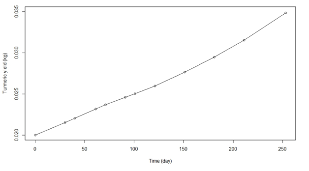
Combining the data of two experiments, we obtain the growth curve of Figure 13 for seed weight 20g. The growth rate is steep after 125 days. We may draw the growth curves of individual’s plants by exponential model as shown in Figure 14 for seed weight 20g. This is of help beyond 253 days when second season starts and auxiliary information is unavailable. The growth slopes are computed, and then increments are computed from the mean of exponential curves; these are sequentially added up to construct the full growth curve. The remaining figures with different seed weights are drawn in a similar fashion see (Figure 15–31). Figure 32 refers to a scaled version of speed in growth curve. In Figure 33 we draw the growth curve based on auxiliary variables for initial seed weight 10g. The adopted procedures are elaborated in figure legends. We notice that growth for seed weight 10g at the end of season 1 is almost 30g. We may thus consider the growth curve of seed weight 30g in season 1 to mimic the remaining part of growth in second season of seed weight 10g. Thus, in a sense, growth curve of turmeric for 10g seed weight is available for the entire time period of two seasons, utilizing auxiliary information. Proliferation rate (d/dt) log y=y1dydt computed in Figure 32–35 is a scaled version of velocity dydt: This measure is independent of the choice of unit used in measuring y=y(t): Computation is based on a technique proposed in Dasgupta,⁴ with exponentially decaying weights attached to empirical slopes computed from data pairs at different time points with respect to a fixed time point t of interest. More weights are given to data points near the time t of derivative computation, and less weight to distant time points from t. Weighted mean of these empirical slopes at derivative stage and smooth. Spine with spar=0.0001 at smoothing stage in S Plus provide proliferation rate at time point t: Proliferation of exponential growth is constant. In Figure 32 we plot the proliferation rate of growth curve of turmeric with seed weight 20g. The curve shows stability near 300 days, the duration of first season, indicating a possibility of exponential growth with parameter 0.0034. During the second season the curve has further drop; deviating from the growth pattern of first season. The rates in Figure 34 of yield based on auxiliary variable, for 10g seed weight indicate that growth is within an exponential band. Variation in the rate over time exhibits a symmetric pattern.

Figure 13 Growth curve from auxiliary information (from all plants): Experiment 1 & 2, season 1 seed wt 20g.

Figure 14 Exponential growth model: Experiment 1 & 2, season 1 & 2 seed wt 20g.

Figure 15 Growth curve: auxiliary information + exponential model, Experiment 1 & 2, season 1 & 2, seed weight 20 g.

Figure 16 Growth curve of 38 plant’s height over 5 time points in season 1, seed weight 10 g.

Figure 16 Effects of P sources and application rates on residual total N in soils after harvest.
Note: P sources ending with 1, 2, 3 and 4 indicates 0, 20, 40 and 60 kg P ha-1 respectively

Figure 17 Growth curve from auxiliary information (from 38 plants): Experiment 1 & 2, season 1 seed wt 10g.

Figure 18 Exponential growth model: Experiment 1 & 2, season 1 & 2 seed wt 10 g.

Figure 19 Growth curve: auxiliary information + exponential model, Experiment 1 & 2, season 1 & 2, seed weight 10g.

Figure 20 Growth curve of 39 plant’s height over 5 time points in season 1, seed weight 15 g.

Figure 21 Growth curve from auxiliary information (from 39 plants): Experiment 1 & 2, season 1 seed wt 15 g.

Figure 22 Exponential growth model: Experiment 1 & 2, season 1 & 2 seed wt 15 g.

Figure 23 Growth curve: auxiliary information + exponential model, Experiment 1 & 2, season 1 & 2, seed weight 15 g 12.

Figure 24 Growth curve of 37 plant’s height over 5 time points in season 1, seed weight 25 g.

Figure 25 Growth curve from auxiliary information (from 37 plants): Experiment 1 & 2, season 1 seed wt 25 g.

Figure 26 Exponential growth model: Experiment 1 & 2, season 1 & 2 seed wt 25 g.

Figure 27 Growth curve: auxiliary information + exponential model, Experiment 1 & 2, season 1 & 2, seed weight 25 g.

Figure 28 Growth curve of 38 plant’s height over 5 time points in season 1, seed weight 30 g.

Figure 29 Growth curve from auxiliary information (from 38 plants): Experiment 1 & 2, season 1 seed wt 30 g.

Figure 30 Exponential growth model: Experiment 1 & 2, season 1 & 2 seed wt 30 g.

Figure 31 Growth curve: auxiliary information + exponential model, Experiment 1 & 2, season 1 & 2, seed weight 30 g.

Figure 32 Proliferation rate of turmeric yield, 20 g.

Figure 33 Growth curve with auxiliary information (from 38 plants): Experiment 1 & 2, season 1 seed wt 10 g.

Figure 34 Proliferation rate of yield on auxiliary variable, 10g.

Figure 35 Proliferation rate of yield on auxiliary + exponential, 10g.

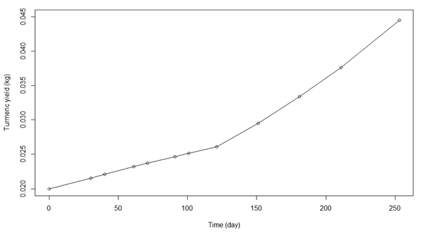
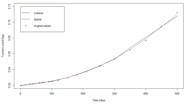
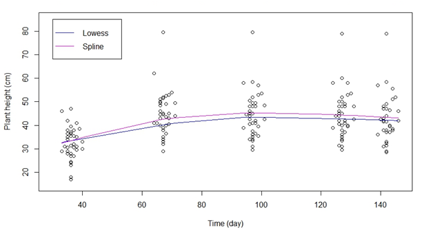
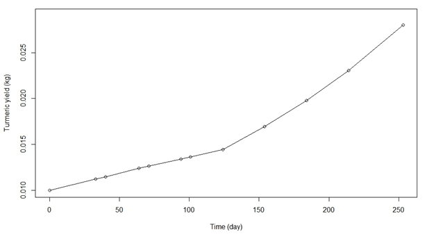
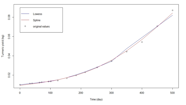
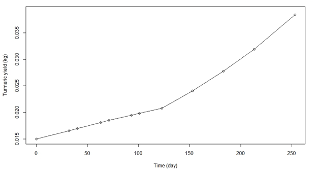
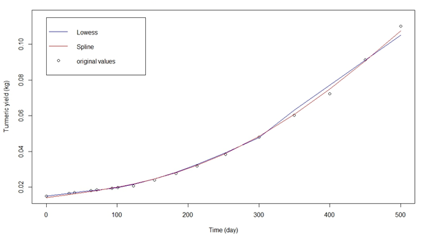
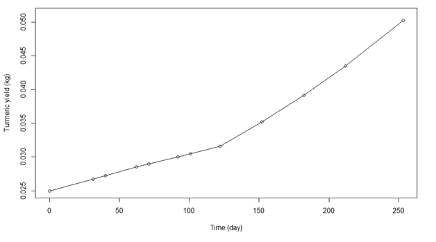
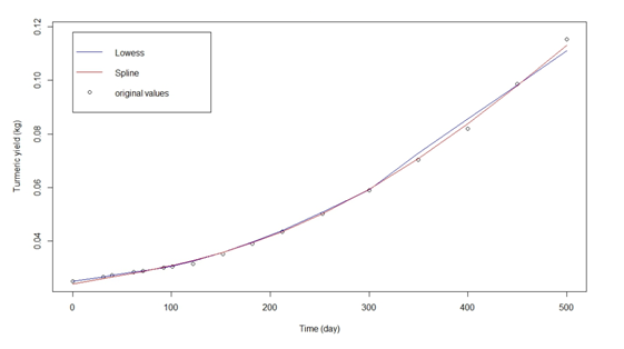
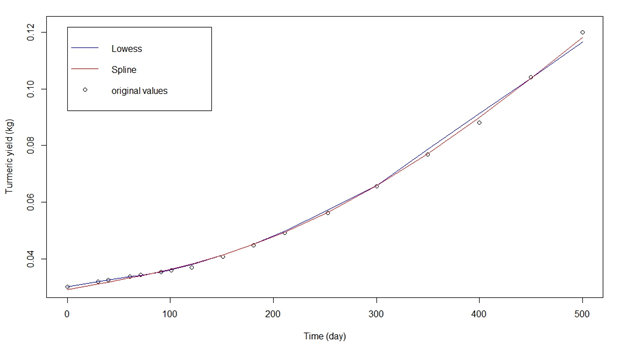
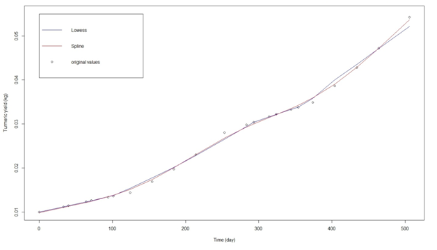
Figure 35 shows the proliferation rate of turmeric yield with seed weight 10g computed from Figure 19, where information from auxiliary variable in season 1 and exponential model in season 2 are used. The curve shows some degree of stability in the time zone [200, 300] days with possibility of exponential growth with parameter 0.00464. The rates shown in Figure 34 and 35 are seen to be different, indicating that auxiliary information have a different role in modeling turmeric yield in comparison to exponential growth model used in season 2. The extended exponential growth model with auxiliary variables is examined for a restricted time period only. In the yam growth experiment, see Dasgupta,⁵ stem height is seen to have a linear relationship with yield in log–log scale.

This is also the case for turmeric growth. Seed weight 10g of turmeric produces best proportionate yield to the tune of 8.71 times in Giridih soil of Jharkhand, when the crop is harvested after second season. Figure 1 For each plant under the experiment with 190 plants, we estimate the yield of a plant with seed weight w; at the end of first season as kw; where an estimate of k² is computed as the ratio of final yield of that plant at the end of second season to the total lifetime of the plant in first and second season together, deleting the dormant period of 107 days in between two seasons. The estimated value of yield kw is linearly regressed by the method of least squares on the maximum plant height of that plant in first season. The value of R² is 0.2732. Linear relationship is apparent in Figure 1, as the lowess curve with f=2/3 is close to the straight line with slope 0.0009041, at the scale of 10^–4: Figure 2. The residuals of regression made in Figure 1 seem to be symmetric around the origin in (Figure 2) (Figure 3). In the log–log scale, we consider the linear regression of yield on max plant height as shown in (Figure 3). The value of R² has slightly increased to 0.2739, compared to the value 0.2732 of Figure 1 in original scale. Figure 4 The residuals of regression made in Figure 3 seem to be asymmetric around the origin in (Figure 4). Figure 5 For each plant at a particular time, we measures length of different leaves in a turmeric plant. Maximum length of leaves in a plant at a time point is recorded.

Maximum of such readings for a plant over time in season 1 is used to regress the yield from that plant at the end of season 1. Figure 5 shows that the linear regression by least square method. The value of R² is 0.1973; lower than 0.2732 of Figure 1 where we considered plant height as independent variable in linear regression. Figure 6 the residuals of regression made in Figure 6 seem to be symmetric around the origin in Figure 6. (Figure 7) In the log–log scale, we consider the linear regression of yield on max leaf length as shown in Figure 7. The value of R² has slightly increased to 0.2147, compared to the value 0.1973 of Figure 1 in original scale. However, this is still less than 0.2739 of Figure 3. (Figure 8) The residuals of regression made in Figure 7 seem to be asymmetric around origin in Figure 8.

Figure 9 Height of 190 plants over experiment 1 & 2 are recorded at ve time points in season 1. These are lowess and spine regressed with parameters f=2/3 and d.f.=3.3 respectively to have overall height growth of plants with time. The growth rate computed from here is of help to assess turmeric tuber growth rate over time via the growth rate of Figure 1. It was not possible to record heights for all the 190 plants in the same day after start. The records are taken over several consecutive days and the points in a group appear like a cluster pillar.

It is possible that the overall plant growth may be attributed to mean of seed weights viz., 20g. We verify this in next picture, (Figure 10). (Figure 10) We may check whether the overall growth pattern of Figure 9 with 190 plants may be attributed to seed weight 20g, the mean seed weight. Figure 10 shows plant height with seed weight 20g for 38 plants over time in season 1. The pattern is almost similar to that of Figure 9 with 190 plants. (Figure 11) At time zero we plot seed weight 20g in the growth curve. For other time points we compute the growth slope as the weighted average of two components, one is the slope from exponential growth, This equals to y₁’(t); where y1(t)=y1(t)=wk^t/506=(total yield from relevant plants at the end of second season)/(total seed weight of relevant plants): There are 19 relevant plants in Experiment 1. The time between two seasons 107 days are deducted from the whole span of two seasons, start to end.

This resulted to lifetime 506 for plants, in general. The other component is computed as growth rate of plant height, as shown in lowess regression of Figure 9. This rate is related to rate of turmeric yield, see Figure 1. A weighted average of the two slopes with weight p=p=10^–4, see Figure 1 asserting that this is the appropriate scale for growth rate of plant height; and the weight (10^–4) for exponential model slope provide the successive increments to the next time point in the growth curve shown in Figure 11, where the points are joined by lines. Figure 12 Following the same technique used in constructing (Figure 11) for Experiment 1, we draw similar picture, (Figure 12); growth curve of turmeric yield over time for Experiment 2 having 19 plants with seed weight 20g. We already mentioned that Figure 9 may represent plant height growth curve over time attributed to mean of seed weights 20g. (Figure 13) We combine plants of Experiment 1 and Experiment 2 with seed weight 20g; there are 38 plants in total.

Following the similar procedure of drawing Figure 11, now with 38 plants; we compute the new value of k to get the turmeric yield growth curve from weighted average of two slopes that provides successive increments to the next time point. The points are joined by straight lines. Figure 14 Individual growth curves of 38 plants in green color are calculated by computing k=final wt=initial seed weight w; for each plant and then using the exponential growth formula y(t)=k^p(t) w; where p(t)=present time t=lifetime. As for example for plant 1, lifetime=500; for plant 2, lifetime=501. The mean curve is computed by calculating the mean value from individual curves at fixed time points. The lowest curve is drawn on those mean points with f=2/3. These two curves are quite close. Figure 15 The growth curve in season 1 is now supplemented by mean curve in exponential growth model shown in Figure 14. The growth increments in time intervals are computed and interpolated from the above mentioned mean curve, and then added after the time zone beyond 253 days when season 1 end.

We calculated the growth slope from mean curve and then added the increment at the last value of season 1 obtained earlier. The lowess curve with f=1/2 and spline regression with d.f=4, over the original values are shown. The growth curves use both auxiliary information and exponential model over the full time span due to nonparametric smoothing. The two curves shown are quite close. Repeating similar procedure, growth curve for different seed weights may be obtained (Figure 16). We consider 38 plants in season 1 for experiment 1 and 2 with seed weight 10g, draw the lowess curve with f=2/3 and spline regression with d.f=3.3 on growth of plant height over time. A similar procedure of drawing Figure 10 with seed weight 20g is followed. (Figure 17) We combine plants of Experiment 1 and Experiment 2 with seed weight 10g; there are 38 plants in total, and follow the similar procedure of drawing Figure 13. We compute the value of k, obtain growth slopes from exponential model and combine this with slope of plant height with appropriate weighting to get the points of growth values in Figure 17. The points are joined by lines (Figure 18). The procedure of drawing Figure 18 is similar to that of Figure 14. Individual growth curves of 38 plants in green color are calculated by computing k=final wt/ initial seed weight w; for each plant and then using the exponential growth formula y(t)=k^p(t)w; where p(t)=present time t/lifetime. As for example for plant number 3 life time is 501.

The mean curve is computed by calculating the mean value from individual curves at fixed time points. The lowest curve is drawn on those mean points with f=2/3: These two curves are quite close. Figure 19 The procedure of drawing Figure 19 with seed weight 10g is similar to that of Figure 15. The growth curve in season 1 is supplemented by mean curve in exponential growth model as shown in Figure 18. The growth increments in time intervals are computed and interpolated from the above mentioned mean curve, and then added in the time zone beyond 253 days when season 1 end. We calculated the growth slope from mean curve and added the increment at the last value of season 1 obtained earlier. The process adding increments is continued to obtain successive points. The lowest curve with f=1/2 and spline regression with d.f=4 over the original values are shown.

The growth curves use auxiliary information and exponential model over life–time from nonparametric smoothing. The two curves shown are quite close (Figure 20). We consider 39 plants in experiment 1 and 2 with seed weight 15g, draw the lowess curve with f=2/3 and spline regression with d.f.=3.3 on growth of plant height over time. A similar procedure of drawing Figure 10 with seed weight 20g and Figure 16 with seed weight 10g is followed (Figure 21). We combine plants of Experiment 1 and Experiment 2 with seed weight 15g; there are 39 plants in total, and follow the similar procedure of drawing Figure 13, Figure 17. We compute the value of k, obtain growth slopes from exponential model and combine this with slope of plant height with appropriate weighting to estimate the turmeric growth in Figure 21. The points are joined by lines. (Figure 22)The procedure of drawing Figure 22 is similar to that of Figure 14, Figure 18. Individual growth curves of 39 plants in green color are calculated by computing k=final wt/initial seed weight w; for each plant and then using the exponential growth formula y(t)=k^p(t) w; where p(t)=present time t/lifetime; and w is the seed weight. The mean curve is computed by calculating the mean value from individual curves at fixed time points. The lowess curve is drawn on those mean points with f=2/3: These two curves are close (Figure 23). The procedure of drawing Figure 23 with seed weight 15g is similar to that of Figure 15, Figure 19.

The growth curve in season 1 is supplemented by mean curve in exponential growth model as shown in Figure 22. The growth increments in time intervals are computed and interpolated from the above mentioned mean curve, and then added in the time zone beyond 253 days when season 1 end. We interpolated the mean curve of Figure 22 at time 350 and 450 days, calculated the growth slope from mean curve and added the increment at the last value of season 1 obtained earlier. The lowess curve with f=1/2 and spline regression with d.f=4 over the original values are shown. The growth curves use auxiliary information and exponential model over lifetime from nonparametric smoothing. The two curves shown are quite close (Figure 24). We consider 37 plants in experiment 1 and 2 with seed weight 25g, draw the lowess curve with f=2/3 and spline regression with d.f=3.3 on growth of plant height over time. A similar procedure of drawing Figure 10 with seed weight 20g, Figure 16 with seed weight 10g, and Figure 20 with seed weight 15g is followed. (Figure 25) We combine plants of Experiment 1 and Experiment 2 with seed weight 25g; there are 37 plants in total, and follow the similar procedure of drawing Figures 13,17,21. We compute the value of k, obtain growth slopes from exponential model and combine this with slope of plant height with appropriate weighting to get the points of growth values in Figure 25.

The points of turmeric yield are joined by lines. Figure 26 The procedure of drawing Figure 26 is similar to that of Figure 14,18,22. Individual growth curves of 37 plants in green color are calculated by computing k=final wt/initial seed weight w; for each plant and then using the exponential growth formula y(t)=k^p(t)w; where p(t)=present time t/lifetime; and w is the seed weight. For example the lifetime for plant 1 with seed weight 25g is 498 days. The mean curve is computed by calculating the mean value from individual curves at fixed time points. The lowess curve is drawn on those mean points with f=2/3: These two curves are close. Figure 27 The procedure of drawing Figure 27 with seed weight 25g is similar to that of Figure 15,19,23. The growth curve in season 1 is supplemented by mean curve in exponential growth model, as shown in Figure 26. The growth increments in time intervals are computed and interpolated from the above mentioned mean curve, and then added in the time zone beyond 253 days when season 1 end. We interpolated the mean curve of Figure 26 at time 350 and 450 days, calculated the growth slope from mean curve and added the increment at the last value of season 1 obtained earlier. The lowess curve with f=1/2 and spline regression with d.f=4 over the original values are shown. The growth curves use auxiliary information and exponential model over lifetime from nonparametric smoothing.

The two curves shown are quite close. (Figure 28) We consider 38 plants in experiment 1 and 2 with seed weight 30g, draw the lowess curve with f=2/3 and spline regression with d.f=3.3 on growth of plant height over time. A similar procedure of drawing Figure 10 with seed weight 20g, Figure 16 with seed weight 10g, Figure 20 with seed weight 15g, and Figure 24 with seed weight 25g is followed (Figure 29). We combine plants of Experiment 1 and Experiment 2 with seed weight 30g, there are 38 plants in total, and follow the similar procedure of drawing Figures 13,17,21,25; originally described in Figure 11.

We compute the value of k = final wt/initial seed weight for each plant, and obtain growth slopes from exponential model and combine this with slope of plant height with appropriate weighting so as to get the points of growth values in Figure 29. The points are joined by lines Figure 30. The procedure of drawing Figure 30 is similar to that of Figure 14,18,22,26. Individual growth curves of 38 plants in green color are calculated by computing k=final wt/initial seed weight w; for each plant and then using the exponential growth formula y(t)=k^p(t)w; where p(t)=present time t/lifetime; and w is the seed weight. For example the lifetime for plant 3 with seed weight 30g is 498 days. The mean curve is computed by calculating the mean value from individual curves at fixed time points. The lowess curve is drawn on those mean points with f=2/3: These two curves are close. We may use these mean values to compute the growth increments.

The procedure of drawing Figure 31 with seed weight 30g is similar to that of Figures 15,19,23,27. The growth curve in season 1 is supplemented by mean curve in exponential growth model, as shown in Figure 30. The growth increments in time intervals are computed and interpolated from the above mentioned mean curve, and then added in the time zone beyond 253 days when season 1 end. We interpolated the mean curve of Figure 30 at time 350 and 450 days, calculated the growth slope from mean curve and added the increment at the last value of season 1 obtained earlier. The lowess curve with f=1/2 and spline regression with d.f=4 over the original values are shown. The growth curves use auxiliary information and exponential model over lifetime from nonparametric smoothing. The two curves shown are quite close (Figure 32). In Figure 32 we plot the proliferation rate of estimated growth curve of turmeric with seed weight 20g with observations from lowess regression shown in Figure 15.

The proliferation curve shows stability near 300 days, the duration of first season, indicating a possibility of exponential growth with parameter 0.0034: During the second season the curve has further drop; showing deviation from the growth pattern of first season Figure 33. So far we have used auxiliary information of season 1 with time range up to 253 days to draw the growth curves. In season 2 for time exceeding 253 days, auxiliary information on plant height and maximum leaf radius are unavailable. However, note that the growth curve with seed weight 10g in season 1 reaches up to 28.01936g at the end of season 1. This is just a little less than the seed weight 30g for which growth data on season 1 is available in association with auxiliary information from Experiment 1 and 2. Thus there is a possibility of translating the growth curve of seed weight 30g in Figure 31 downward in Y axis by pulling it down by that small amount of gap and merge this with growth curve of turmeric seed weight 10g to the end of season 1, to have an overall representation of growth curve with seed weight 10g over two seasons extending up to 500 days. Hence we obtain Figure 33 representing growth curve of 10g turmeric seed weight over a time span of 500 days covering two seasons and utilizing auxiliary information of plant height throughout, in spite of limited data available.

Here we use lowess (f=2/3) and spline regression (df=6) over data points. The yield growth seems higher in the second sprouting in cultivation (Figure 34). In (Figure 34) we compute the proliferation rate of yield from the data points shown in Figure 33. Proliferation of exponential growth is constant. The rates in Figure 34 indicate that turmeric growth is within an exponential band. Variation in the proliferation rate over time exhibit a symmetric pattern, like a periodic function in upper and lower halves in Y axis around time 250 days. Figure 35 shows the proliferation rate of turmeric yield with seed weight 10g computed from Figure 19, where information from auxiliary variable in season 1 and exponential model in season 2 are used. The curve shows some degree of stability in the time zone [200, 300] days with possibility of exponential growth with parameter 0.00464. We may compare the proliferation rate shown in Figure 34 for seed weight 10g based mainly on auxiliary variables, with proliferation rate for same seed weight shown in Figure 35 and computed from growth curve of Figure 19, where turmeric growth is computed using auxiliary information in season 1, and exponential model in season 2. The rates shown in Figures 34 & 35 are seen to be different, indicating that auxiliary information incorporates modification in modeling turmeric yield.

The exponential growth curve y(t)=(1+c)^t y(0) has a linear relationship in the log scale, log y(t)=t log (1+c)+log y(0). For c<0 the curve shows exponential decay. Now, consider c=c_t to be such that –1<a=lim inf ct < lim sup c_t=b<1. Then for |c|<1, t log (1+c) ≈ t (c–c² /2+c³ /3 – ...) and variation of y (t) is in between a band of two exponential curves. Conversely, if the variation of y(t) is in between a band with two exponential curves then –1<a=lim inf c_t<lim sup c_t=b<1 for some a; b holds, where c=c_t=[y(t)/y(0)]^1/t g1=t. In discrete case let t ɛ Ν₀={0, 1, 2, 3, ...}g, then the condition remains the same for an exponential band to contain the growth curve. The above assertion is on growth curve lying in a band involving upper and lower exponential growth bounds. A stronger assertion on convergence of y(t) to an exponential growth curve is possible if b=c; when the band merges to a curve. Some special cases considered in Dasgupta⁶ are revisited below. Proliferation rate d td log y (t) determines a growth curve y=y(t) when initial value is specified. For exponential growth this rate is a constant. Discrete version of growth is considered in Dasgupta.⁶

Some discrete version of unbounded growth models

The growth observations are taken on discrete time points with unequal spacing. In a bounded time zone, the growth may exhibit exponential rate. In view of the relationship of proliferation rates among growth curve families in continuous time, one may consider discrete version ∆y(t)/ {y(t) ∆t}tg of the three proliferation rates given in (2) of Dasgupta⁶ that gives rise to the discrete growth curves for t ɛ Ν₀={0, 1, 2, 3, ...} ::: g satisfying the following difference equations.

∆y(t)/ {y(t) ∆(t)} y(t+1)/y(t) –1=cνβ[1– exp({(1/y(t))^1/ν–1}/β)]→ cν{1–(1/y(t))^1/ν}, β → ∞; this converges to – c log (1/y(t)) as ν → ∞ ...(3)

That is, for t ɛ Ν₀={0, 1, 2, 3, ...} ::: g

y(t+1)=[1+cνβ[1– exp({(1/y(t))^1/ν –1}/β)]]y(t) ...(4)

y(t+1)=[1+cν{1–y(t)^–1/ν}] y(t)...(5)

y(t+1)=[1+c log y(t)]y(t) ...(6)

For unbounded growth observations recorded at discrete time, the above family of models (4)–(6) with some assigned initial value for y(0)>1 may be appropriate. The findings are true for unequal spacings, similar limit holds in (3). That is y(t+1) on the l.h.s of (3)–(6) are to be replaced by y(t+Δ(t)) and the r.h.s of these equations has to be multiplied by a factor Δ(t), the unequal time spacing. The proofs are similar. When the limits are achieved in (3)/(5) for proliferation rates in discrete case with unequal spacing Δ=Δ(t), discrete version of exponential distribution is attained, for example when c=c_t=c*/log y(t). This family of discrete proliferation rates, like its continuous time counterpart, covers a broad spectrum starting from exponential to logarithmic order of growth in a continuous manner, as the next class in the series (4)–(6) is a limit of the former. The growth curve given in (3)/ (5) has a proliferation converging to a constant c for large time. Some figures on proliferation rates computed in the present context of turmeric growth showed stability towards a constant, justifying exponential model in a limited zone. An exponential growth will overcome linear or any polynomial growth in time. Then equation (3)/ (5) will result in the discrete or continuous version of exponential growth in the limit.

The growth experiment was conducted to see the effect of different seed weights 10g, 15g, 20g, 25g and 30g on turmeric yield. The experiment was repeated in two adjacent plots in a season and prolonged up to the end of second season. Experiments continued in same pits over a period of two seasons to obtain high yield at the end of second season. Farmers often take recourse to this standard practice in anticipation of a good harvest. Turmeric plants sprouted for a second time in same pits in second season as the crop remained unharvested at the end of first season. Yield data is available only at the end of second season. Problem is to identify the appropriate seed weight, the growth curve of yield, and the best linear predictor based on above ground auxiliary variables in usual or in log–log scale for yield over extended time of cultivation.

Seed weight 10g of turmeric is seen to produce best proportionate yield to the tune of 8.71 times at the end of second season in lateritic alluvial soil of Giridih, Jharkhand (India). Above ground auxiliary variables on biomass like maximum leaf length and plant height are recorded only for the first season due to resource constrains. An exponential model in the first season is taken from elementary consideration of proportionate growth, assuming yield at harvest is a multiple of seed weight; the multiplicative constant for each plant is then estimated from final harvest of the plant. From the limited data on auxiliary variables, growth curve of yield is obtained in section 2 by least squared regression, nonparametric smoothing of lowess and spline, along with a modification of exponential model under the consideration of proportionate growth in yield over time. Of all the variables considered, seed weight, lifetime and plant height are seen to be significant in analysis of variance.

The best linear predictor is obtained in Equation (1), and this is validated for different pro les of plant lifetime. Maximum plant height is seen to be a good predictor of the yield and this variable is used to calibrate the exponential growth model. The proposed procedure blends the information from observable auxiliary variable with yield data available at the end of second season. Proliferation rate of exponential growth is constant. The growth curve of turmeric yield show such a property toward end of the first season. In earlier yam growth experiments, see e.g., Dasgupta,⁵ stem height is seen to have a linear relationship with yam yield in log–log scale. The same is observed for turmeric growth. Accuracy of prediction is higher in log–log scale. Farmers may use seed weight 10g of turmeric that produces best proportionate yield to the tune of 8.71 times in the soil of Giridih Jharkhand, when turmeric is harvested after the second season; the growth is seen to be faster in the second season.

The paper is dedicated to the memory of late Professor Jayanta K Ghosh, former director of the Indian Statistical Institute. Professor Ghosh inspired the author on theory cum applied work.

The author declares no conflict of interest.

1. Holt PR, Katz S, Kirsho R. Curcumin therapy inflammatory bowel disease: a pilot study. Dig Dis Sci. 2005;50(11):2191–2193.
2. Dasgupta R. Optimal Choice of Small Regular Shapes for Accidentally Damaged Tessellation. Chapter 15, In: Growth Curve and Structural Equation Modeling: Topics from the Indian Statistical Institute, Springer, Germany; 2015. p. 287–299.
3. Slavov N, Budkin BA, Schwab D, et al. Constant growth rate can be supported by decreasing energy flux and increasing aerobatic glycolysis. Cell Rep. 2014;7(3):705–714.
4. Dasgupta R. Rates of Convergence in CLT for Two Sample U Statistics in Non iid Case and Multiphasic Growth Curve. In: Growth Curve and Structural Equation Modeling. Dasgupta R, editor. Springer Proceedings in Mathematics & Statistics. 2015. 132:35–58.
5. Dasgupta R. Yam Growth Experiment and Above-ground Biomass as Possible Predictor. In: Advances in Growth Curve Models: Topics from the Indian Statistical Institute, Chapter 1, Springer Proceedings in Mathematics & Statistics, 46, Switzerland; 2013. p. 1–33.
6. Dasgupta R. Unbounded Growth Model for Word Frequencies in Political Transition. In: Growth Curve and Structural Equation Modeling: Topics from the Indian Statistical Institute. Chapter 12, Springer, Germany; 2015. p. 209–221.