Research Article Volume 13 Issue 4
A compound of exponential and Komal distributions with properties and application
Dr. Rama Shanker,
shankerrama2009@gmail.com
Mousumi Ray
Correspondence: Dr. Rama Shanker, Department of Statistics, Assam University, Silchar, India
Received: October 28, 2024 | Published: November 22, 2024
Citation: Ray M, Shanker R. A compound of exponential and Komal distributions with properties and application. Biom Biostat Int J. 2024;13(5):147-152 DOI: 10.15406/bbij.2024.13.00425
Download PDF
Abstract
In this paper exponential-Komal distribution, the compound of exponential distribution with Komal distribution has been proposed. The key feature of the proposed compound distribution is that it doesn't have a moment generating function or moments which might seem like a limitation, but this distribution can be very much useful for modelling data from biomedical sciences and engineering of heavy tailed behaviour. Important statistical properties of the distribution have been studied. The estimation of its parameter has been discussed using maximum likelihood method. Goodness of fit of the proposed distribution has been explained with an example of real life data having decreasing failure rate. The fit has been found quite satisfactory over exponential, Lindley, Shanker, Komal, exponential-Lindley and exponential-Shanker distributions.
Keywords: lifetime distribution, statistical properties, stress-strength reliability, maximum likelihood estimation, goodness of fit.
Introduction
In the realm of distribution theory one parameter exponential distribution and Lindley distribution given by Lindley1 are popular. Both exponential and Lindley distributions are useful for modelling different types of random events, particularly those that involve waiting times, failure times, or life spans, but Lindley provides more flexibility when the assumptions of the exponential model are too strict. A comparative study of exponential and Lindley distribution done by Shanker et al2 found that in certain datasets exponential outshines while in others, the Lindley offers a more precise fit and also there were some datasets where both the distributions aren’t provides optimal fit. Highlighting the need for more flexible models, Shanker3 proposed a new one parameter lifetime distribution named Shanker distribution which provides much better fit than both exponential and Lindley distributions. Shanker4 proposed another one parameter lifetime distribution called Komal distribution which provides much better fit than Shanker, exponential and Lindley distributions. The Komal distribution is defined by its probability density function (pdf) and cumulative distribution function (cdf)
(1)
(2)
Komal distribution is a two- component mixture of exponential
distribution and a gamma
distribution with mixing proportion
and
respectively. Recently, Shanker et al5,6 derived the weighted version and the power version of Komal distribution respectively.
Belhamra et al7 proposed the compound of exponential and Lindley distribution and named exponential-Lindley distribution (E-LD) having pdf and cdf
(3)
(4)
Recently, Ray and Shanker8 proposed a compound distribution namely exponential-Shanker distribution (E-SD) and discussed its various statistical properties, estimation of parameter and application for engineering data and showed that it provides much closer fit than other compound distributions. The E-SD is defined by its pdf and cdf
(5)
(6)
Both the E-LD and the E-SD is a particular cases of gamma- Lindley distribution (G-LD) of Abdi et al9 and gamma-Shanker distribution (G-SD) by Ray and Shanker10 respectively.
The main purpose for introducing the compound of exponential and Komal distribution are that the compound distributions are much useful for the study of heterogeneous population which is the reality of present real life situations and to examine its fit over other compound distributions. Further, as we know that Komal distribution provides much closer fit than exponential, Lindley and Shanker distributions, it is expected that the compound of exponential and Komal would provide much closer fit over the compound of exponential and Lindley distributions and the compound of exponential and Shanker distributions. Statistical properties, estimation of parameter and application of the proposed distribution have been discussed. One of the most important advantages of compounding exponential and Komal distribution is that the hazard rate for exponential distribution is constant but the hazard rate for the compound of exponential and Komal distributions is not constant but it is decreasing. Further, although the moment generating function and the moments of the proposed distribution do not exist, but the distribution is very much useful to model data of heavy tailed behaviour.
Exponential - Komal distribution
The pdf and the cdf of the compound of exponential and Komal distribution named exponential-Komal distribution (E-KD) are obtained as
(7)
(8)
The shapes of the pdf and the cdf of E-KD for varying values of parameter are shown in the following 1and 2 respectively. For better visualization of the plots of cdf we used 3D plots of the same in the 3.
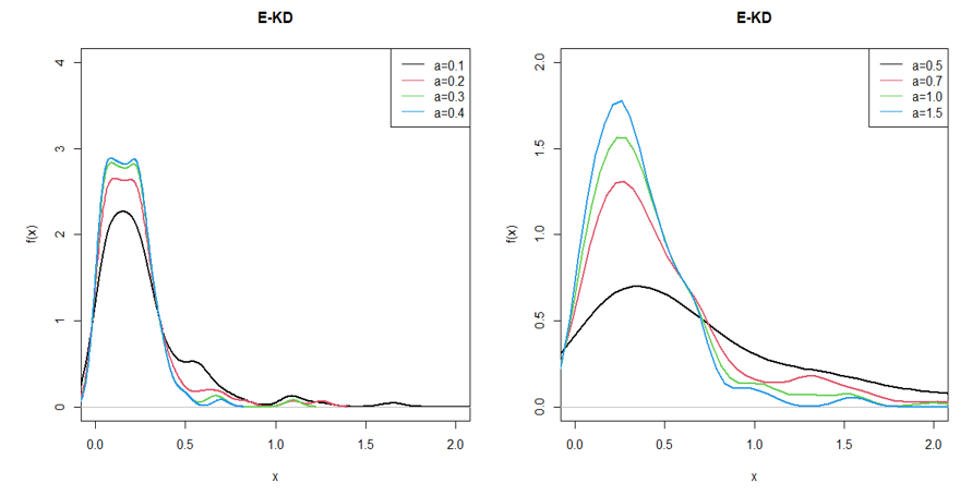
Figure 1 Pdf of E-KD for some selected values of parameter.
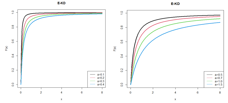
Figure 2 Cdf of E-KD for some selected values of parameter.
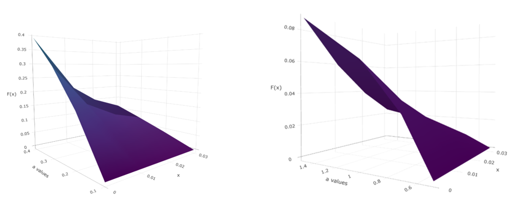
Figure 3 3D plots of cdf of E-KD for some selected values of parameter.
Theorem 1: The pdf of E-KD distribution is decreasing for .
Proof: We have,
,
Where, C is a constant. We have
For
,
and this means that
is decreasing for all
.
Hazard function and reversed hazard function
The hazard function and the reversed hazard function are two important functions of a distribution. The reliability (survival) function of E-KD can be obtained by
(9)
The corresponding hazard function and reversed hazard function of E-KD are obtained as
(10)
(11)
The behavior of
when
and
, respectively are
and
and
.
The shapes of the hazard function and the reversed hazard function of E-KD for varying values of parameter are shown in the following 4 and 6 respectively. Also, for better visualization of the plots of the hazard function and the reversed hazard function, we used 3D plots of the same in the 5 and 7 respectively.
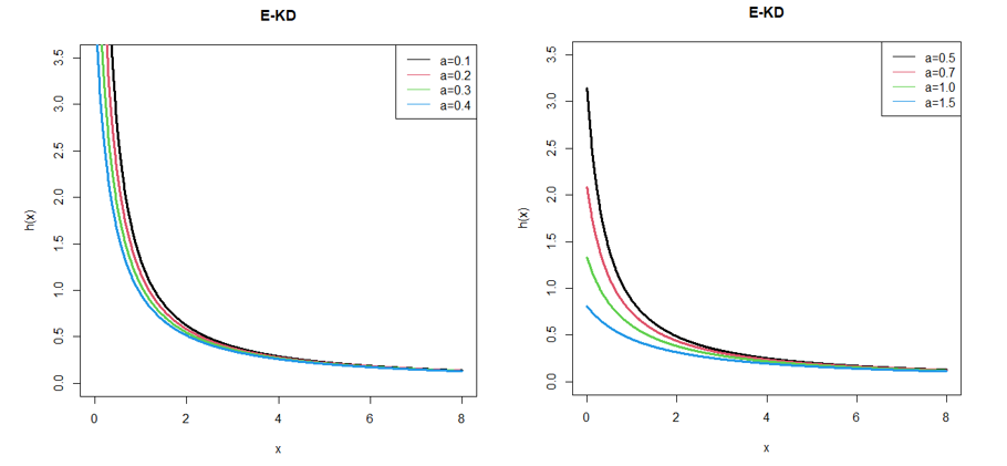
Figure 4 Hazard function of E-KD for some parameter values.
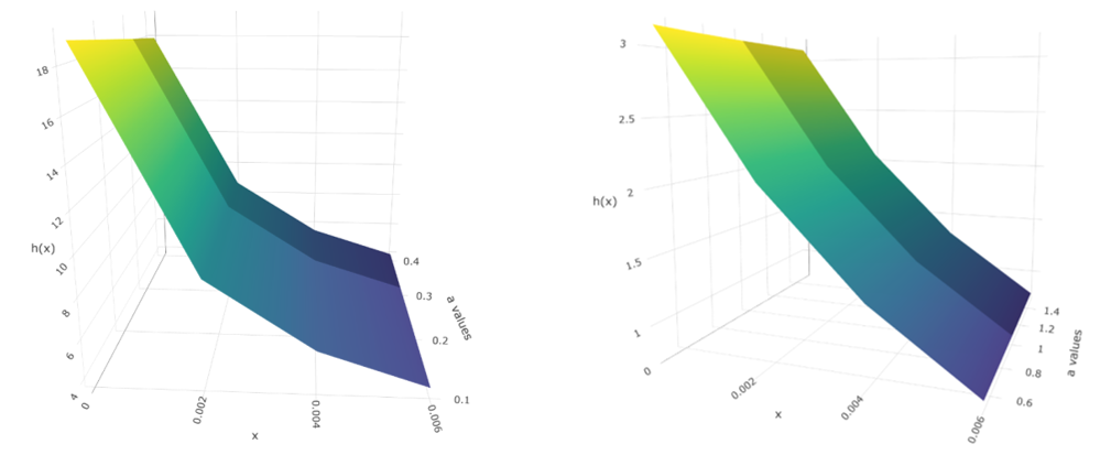
Figure 5 3D Plots of hazard function of E-KD for some parameter values.
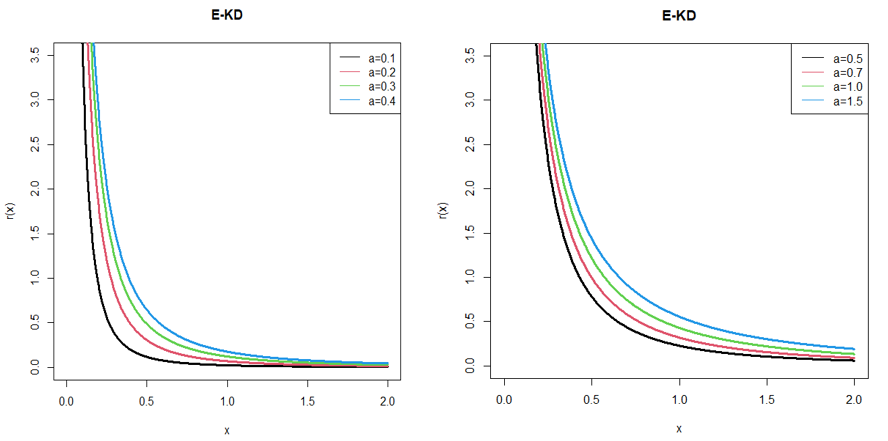
Figure 6 Reversed hazard function of E-KD for some parameter values.
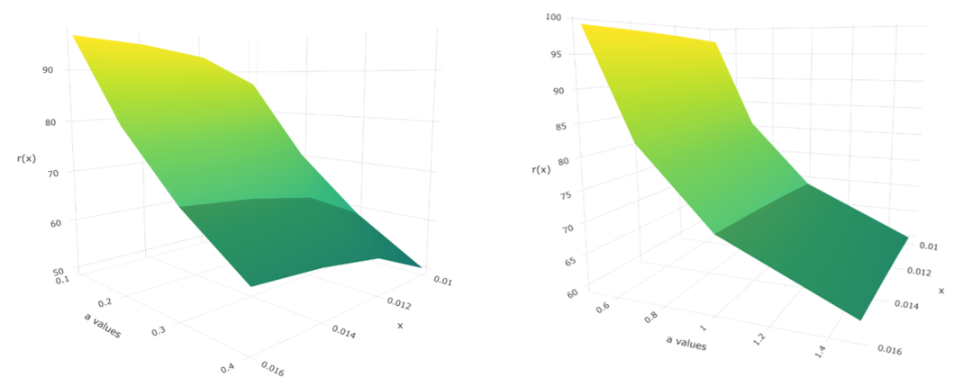
Figure 7 3D Plots of reversed hazard function of E-KD for some parameter values.
Theorem 2: The hazard function of the E-KD is decreasing
Proof: We have
Now, suppose that
.
This gives
Theorem 3: The reversed hazard function of the E-KD is decreasing
Proof: We have,
This gives
for all
Quantiles and moments
The pth quantiles
of E-KD defined by
, is the root of the equation
This gives
(12)
It should be noted that this
may be used to generate E-KD random variates. Further, the median of E-KD can be obtained from above equation by taking
.
The moments and the moment generating function of E-KD do not exit and it has been shown mathematically in the following theorems 4 and 5 respectively.
Theorem 4: The moments of the E-KD does not exist.
Proof: The
moment of E-KD is given by
Let,
. As
we have
Using beta integral of second kind
, we get
Here the range is
but
. Hence
does not exist.
Theorem 5: The moment generating function of the E-KD does not exist.
Proof:
Now, we have
At,
integral function is unbounded in the neighborhood of ,
so
is divergent . This means that moment generating function does not exist
Entropies
Renyi entropy
Renyi entropy, proposed by Renyi11 measures the variation of uncertainty in the distribution. The Renyi entropy is defined as
Where
(13)
Applying binomial expansion
, we get
Where,
(14)
Tsallis entropy
Tsallis12 introduced entropy called Tsallis entropy for generalizing the standard statistical mechanics which is defined as
(15)
Applying binomial expansion
, we get
(16)
Extreme order statistics
Let,
be the order statistics of a random sample of size n from the E-KD (a) distribution with distribution function F(x). The cdf of the minimum order statistic
is given by
The cdf of the maximum order statistic
is given by
Stochastic orderings
Stochastic ordering is used to compare two lifetime distributions to examine how one variable is greater than the other.
A random variable X is said to be smaller than a random variable Y in the
- Stochastic order
if
for all x
- Hazard rate order
if
for all x
iii. Mean residual life order
if
for all x
- Likelihood ratio order
if
decrease in x
The following results due to Shaked and Shanthikumar13 are well known for establishing stochastic ordering of distributions:
Theorem 6: Let
and
.If
then
.
Proof: We have
Let,
,
Where,
For
,
.This means that
and hence
and
.
Estimation of parameters
Let
be the observed values of a random sample
from the E-KD. Then the Likelihood function is given by
(17)
The log-likelihood function of E-KD is thus obtained as
(18)
The maximum likelihood estimate of the parameter is the solution of the following log-likelihood equation
(19)
It can be easily shown that the maximum likelihood estimate will satisfy the second order sufficient condition of maximum likelihood estimator. For, we have
(20)
Estimation of the stress-strength parameter
In reliability, the stress-strength model describes the life of a component which has a random strength X subjected to a random stress Y.The component fails at the instant if the stress applied to it exceeds its strength, and the component will function satisfactory whenever,X>Y. In this section our objective is to estimate
when
and
and X and Y are independently distributed. Thus, the stress- strength parameter is given by
= H
Let,
be the observed value of a random sample of size from E-KD
and
be the observed value of a random sample of size m from E-KD
.
The log-likelihood functions of
and
is given by
The maximum likelihood estimates of and are the solutions of following log-likelihood equations
Solving these non-linear equations using any iterative methods available in R packages we can obtain the MLEs of the parameters as
and hence the MLE of R can thus be obtained as
H
.
A simulation study
This section contains a simulation study to examine the consistency of maximum likelihood estimator of the parameter of the E-KD. The mean, bias (B), MSE and variance of the MLE’s are computed using the formulae
,
,
,
Where,
and
.
The simulation results of E-KD have been presented in table 1 using acceptance-rejection method of simulation.
|
Parameters
|
Sample Size
|
Mean
|
Bias
|
MSE
|
Variance
|
|
|
20
|
1.482652
|
-0.0173482
|
0.000865
|
0.000564
|
|
40
|
1.486166
|
-0.0138335
|
0.000719
|
0.0005279
|
|
60
|
1.484523
|
-0.0154774
|
0.000537
|
0.0002981
|
|
80
|
1.482652
|
-0.0114015
|
0.000468
|
0.0003381
|
|
100
|
1.482957
|
-0.0100429
|
0.000444
|
0.000344
|
Table 1 The mean, biases, MSE and variances of E-KD for
Application
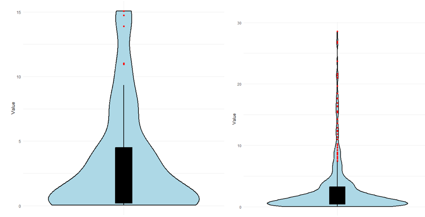
This section deals with the goodness of fit of E-KD over E-LD, E-SD, Shanker, Komal, Lindley and exponential distributions. The applications and the goodness of fit have been presented with one real dataset relating to failure times of 50 components. The summary of the dataset is presented in table 2. The total time to test (TTT) plots and Violin plot of the dataset related to failure times and simulated dataset are given in 8 and 9 respectively. The goodness of fit of the considered distributions for the dataset is provided in table3. The fitted plots of the considered distributions for the dataset are given in 10. The dataset is as follows:
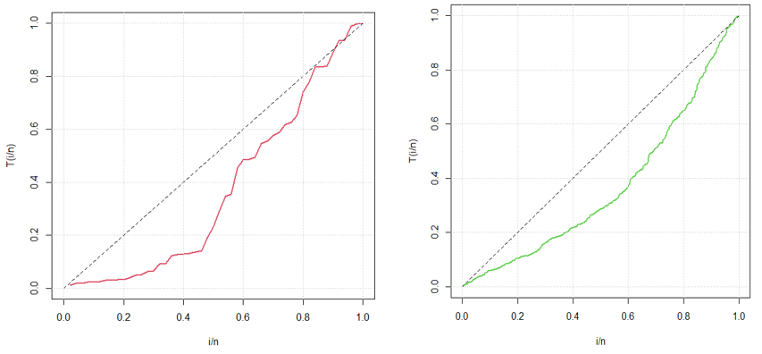
Figure 8 TTT-plot of dataset and simulated dataset related to failure times of E-KD.

Figure 9 Violin-plot of the dataset related to failure times and simulated data of E-KD respectively.
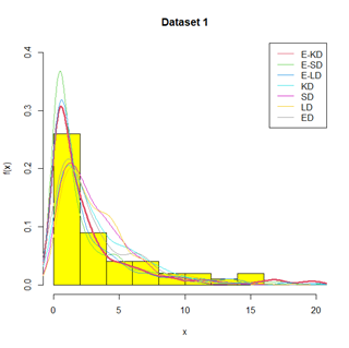
Figure 10 Fitted plots of distributions for the dataset 1.
Dataset 1: The following extreme skewed to right data, discussed by Murthy et al14 presents the failure times of 50 components and the observations are:
0.036, 0.058, 0.061, 0.074, 0.078, 0.086, 0.102, 0.103, 0.114, 0.116, 0.148, 0.183, 0.192, 0.254, 0.262, 0.379, 0.381, 0.538, 0.570, 0.574, 0.590, 0.618, 0.645, 0.961, 1.228, 1.600, 2.006, 2.054, 2.804, 3.058, 3.076, 3.147, 3.625, 3.704, 3.931, 4.073, 4.393, 4.534, 4.893, 6.274, 6.816, 7.896, 7.904, 8.022, 9.337, 10.940, 11.020, 13.880, 14.730, 15.080
|
Min
|
1st Qu.
|
Median
|
Mean
|
Variance
|
3rd Qu.
|
Max
|
|
0.036
|
0.2075
|
1.414
|
3.343
|
17.48477
|
4.4988
|
15.08
|
Table 2 Summary of the dataset 1
|
Distributions
|
ML estimates and standard error
|
|
AIC
|
K-S
|
P- value
|
|
E-KD
|
1.4566 (0.2932)
|
211.9573
|
213.9573
|
0.1423
|
0.3202
|
|
E-SD
|
1.5819 (0.2822)
|
212.1365
|
214.1365
|
0.1614
|
0.1887
|
|
E-LD
|
1.7208 (0.3529)
|
212.3744
|
214.3744
|
0.2769
|
0.0009
|
|
KD
|
0.4847 (0.0483)
|
234.9971
|
236.9971
|
0.3093
|
0.0003
|
|
SD
|
0.5713 (0.0509)
|
249.9203
|
251.9203
|
0.3454
|
0
|
|
LD
|
0.4987 (0.0513)
|
240.3559
|
242.3559
|
0.3469
|
0
|
|
ED
|
0.2991(0.0423)
|
220.6857
|
222.6857
|
0.28
|
0.0097
|
Table 3 Goodness of fit of E-KD along with other distributions for dataset 1
Concluding remarks
In this paper, we introduced exponential-Komal distribution (E-KD) by compounding exponential distribution with Komal distribution. Several key characteristics of this distribution have been thoroughly explored, including its shape, hazard and reversed hazard functions, quantile function, Rényi entropy, Tsallis entropy and stress-strength reliability. Maximum Likelihood estimation has been discussed for estimating its parameter. The goodness of fit of E-KD over E-LD, E-SD, Komal distribution, Shanker distribution, Lindley distribution and exponential distribution shows that E-KD gives much closer fit than these distributions for the dataset related to failure times of 50 components.The proposed distribution is very much useful for modelling data from biomedical sciences and engineering having heavy tailed behaviour.
Acknowledgments
Authors are grateful to the editor in chief of the Journal and the anonymous reviewer for some fruitful comments which improved the quality of the paper.
Conflict of interests
The authors declare that there are no conflicts of interest.
References
- Lindley DV. Fiducial distribution and Bayes’ theorem. J R Statist Soc.1958;20(1):102–107.
- Shanker R, Hagos F, Sujatha S. On modelling of lifetimes data using exponential and lindley distributions, Biom biostat int. 2015;2(5):140–147.
- Shanker R. Shanker distribution and its applications, International Journal of Statistics and Applications, 2015;5(6):338–348.
- Shanker R. Komal distribution with properties and application in survival analysis. Biom Biostat Int J. 2023;12(2):40–44.
- Shanker R, Ray M, Prodhani HR. Weighted Komal distribution with properties Shanker and applications, Int J Statist and Relia Eng. 2023a;10(3):591–603.
- Shanker R, Ray M, Prodhani H R. Power komal distribution with properties and application in reliability engineering. Relia Theo App. 2023b;18(4):541–551.
- Belhara T, Zeghdoudi H, Raman V. A new compound exponential lindley distribution application and comparison. Int J Agri Statist sci. 2022;18(2):755–766.
- Ray M, Shanker R. A compound of exponential and Shanker distribution with an application. J Sci R. 2023a;67(4):39–46.
- Abdi M, Asgharzadeh A, Bakouch HS, et al. A new compound Gamma and Lindley distribution with application to failure data. Austrian J Statist. 2019;48:54–75.
- Ray M, Shanker R. A compound of Gamma and Shanker distribution. Relia Theo App. 2023b;18(2):87–99.
- Renyi A. On measure of entropy and information. In: proceeding of the fourth Berkeley symposium on mathematical statistics and probability. Contribution to the theory of Statistics, Berkeley, California: University of California Press. 1961;(1):547–561.
- Tsallis C. Possible generalization of Boltzmann- Gibbs statistics. J Statist Phy. 1988;52(1-2):479–487.
- Shaked M, Shanthikumar JG. Stochastic orders and their applications. Academic Press New Work.1994.
- Murthy D N P, Xie M, Jiang R. Weibull models. John Wiley & Sons Inc, Hoboken. 2004:416.

©2024 Ray, et al. This is an open access article distributed under the terms of the,
which
permits unrestricted use, distribution, and build upon your work non-commercially.


