We study the behavior critical of the Potts model with 3 states on Solomon networks using Monte Carlo simulations. Our results show that this presents a first-order phase transition. These results are different of the Potts model with 3 states on a square lattice that present a second-order phase transition. However, these are consistent with the results of the Potts model on Erdös–Rényi random graphs.

Keywords: potts, networks, spins

The Ising model is useful to simulate the behavior of people in a community, where each person can be influenced by the neighbors, or influences these neighbors. However, the neighbors at home differ from the neighbors in the workplace except when everybody works at home. Thus the home neighborhood and the workplace neighborhood can be approximated by using two chains of L sites each, the home chain and the workplace chain. In the workplace chain, the people are numbered consecutively from i=1 to i=L with toroidal boundary conditions. So the same people i also appear in the home chain but in different order P(i), which is a random permutation of the order in the workplace chain. Thus each person has exactly one place in the home chain, and each site in the home chain is occupied by exactly one person, just as the case for the workplace chain. The same person occupies two entirely different sites i and P(i) in the two chains of L size lattice with N=2L sites.

Such a network of two lattices (in our case two chains) is called a Solomon network.¹ In these networks each person is equally shares by two lattices, just as in the biblical story of King Solomon; also the model was suggested by Sorin Solomon^2,3 Within each chain we have the usual type of interaction like Ising, MVM, Sznajd model and others and added to it the interaction of each person with the neighbors of its own image in the other chain. Thus in a chain of people i with nearest neighbor interaction, the variables at site i interacts with the variable at sites $i\pm \text{1}$  as well as with the neighbors $P\left(i\right)\pm \text{1}$  of the site P(i) of the other chain, where P is the permutation of the numbers i =1, 2, . . . , N.

This Solomon network is close to small-world networks.^4,5 One could, of course, introduce some correlation between residence and workplace, making P(i) not completely random when people select works closer to their homes. We do not discuss here higher-dimensional lattices instead of our chains.

The Potts model in two-dimension (d=2) present phase transition at finite temperature T, for any number of states q. However in d=2 there are a second-order phase transition and a first-order transition $q\le \text{4}$ and $q\ge \text{5}$ , respectivelly.⁶

Silva et al.,⁷ have studied through Monte Carlo simulations a two-dimensional Potts models with q=3 and q=4 states on a directed small-world network. From this study they found both, a first-order and second order phase transition for q=3 depending on the rewiring probability p. Otherwise, for q=4 the system shows only a first-order phase transition for any value of a rewiring probability p.

Recently, Lima FWS⁸ studied the three-states ferromagnetic Potts model on Erdös-Rènyí random graphs.⁹ Their results showed that this model presents only a first-order phase transition. In this paper we consider the Potts model with q=3 states on Solomon networks (Sns). On this system, we perform a set of Monte Carlo simulations using the spin-flip heat bath algorithm to update the spins.

The time evolution of the system is given by a single spin-flip like dynamics⁶ with a probability described by

$P_i=\text{1}/\left[\text{1}+\text{exp}\left(\text{2}{E}_i/K_{B}T\right)\right]$     (1)

Where T is the temperature,  is the Boltzmann constant, and  is the energy of the configuration obtained from

$E_i=-J{\displaystyle \sum _{\text{j=1}}^k{\delta }_{S_i{S}_j}}$     (2)

Where the sum is carried out over the k neighbors of site i. In the above equation J is the exchange coupling. The simulations have been performed on different SNs comprising a number N=2000, 10000, 20000, 40000, 60000, 80000, 120000 and 160000 of sites. For each system size quenched averages over the connectivity disorder are approximated by averaging over independent realizations. For each simulation, we have started with a uniform configuration of spins. We ran $\text{3}x{\text{10}}^{\text{5}}$ Monte Carlo steps (MCS) per spin with $\text{2}x{\text{10}}^{\text{5}}$ configurations discarded for thermalization using the “perfect” random-number generator.¹⁰ We do not see any significant change by increasing the number of replicas (R) (for example R=50 ) and MCS. So, we keep these values constant once they seem to give reasonable results for all simulations.

Here, we have employed the heat bath algorithm¹¹ and for every MCS, the energy per spin, e=E/N, and the magnetization per spin, m=M/N with M=(q. max[]-N)/(q-1), were evaluated. Where $n_i\le N$ denotes the number of spins with "orientation" i=1,...,q.

From the energy measurements we can compute the average energy, specific heat, and also the fourth-order Binder cumulant of the energy, given respectively by

$u\left(T\right)={\left[\langle e\rangle \right]}_{\text{av}}/N$ ,     (3)

$C\left(T\right)=\frac{N}{T^{\text{2}}}\left({\left[\langle e^{\text{2}}\rangle \right]}_{\text{av}}-{\left[{\langle e\rangle }^{\text{2}}\right]}_{\text{av}}\right)$ ,     (4)

$B_e\left(T\right)=\text{1}-\frac{{\langle e^{\text{4}}\rangle }_{\text{av}}}{\text{3}{\left[\langle e\rangle \right]}_{\text{av}}^{\text{2}}}$ .     (5)

In the above equationsstands for thermodynamic averages ${\left[\mathrm{...}\right]}_{\text{av}}$ and for averages over different realizations. Similarly, we can derive from the magnetization measurements the average magnetization, the susceptibility, and the fourth-order magnetic cumulant,

$m\left(T\right)={\left[\langle \left|m\right|\rangle \right]}_{\text{av}}$ ,     (6)

$\chi \left(T\right)=\frac{N}{T}\left({\left[\langle m^{\text{2}}\rangle \right]}_{\text{av}}-{\left[{\langle m\rangle }^{\text{2}}\right]}_{\text{av}}\right)$ ,     (7)

$U_{\text{4}}\left(T\right)=\text{1}-\frac{{\langle m^{\text{4}}\rangle }_{\text{av}}}{\text{3}{\left[\langle m\rangle \right]}_{\text{av}}^{\text{2}}}$ ,     (8)

A more quantitative analysis can be carried out through the FSS of the specific heat $C_{\text{max}}$  , the susceptibility maxima ${\chi }_{\text{max}}$ and the minima of the Binder parameter $B_{\text{i,min}}$ . If the hypothesis of a first-order phase transition is correct, we should then expect, for large system sizes, an asymptotic FSS behavior of the form,^12,13

$C_{\text{max}}{\text{=a}}_C{\text{+b}}_C\text{N+}\mathrm{...}$     (9)

${\chi }_{\text{max}}{\text{=a}}_{\chi }{\text{+b}}_{\chi }\text{N+}\mathrm{...}$     (10)

$B_{\text{i,min}}{\text{=a}}_{B_i}{\text{+b}}_{B_i}/\text{N+}\mathrm{...}$     (11).

The $B_e\left(T\right)$ (equation (5)) also known as the Binder parameter, gives a qualitative as well as a quantitative description of the order of the transition. It is known¹³ that this parameter takes a minimum value $B_{\text{i,m}}$ at the effective transition temperature. 

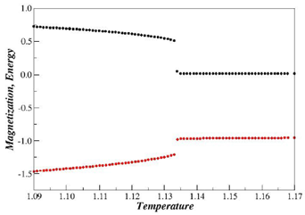
In the Figure 1, we plot the magnetization and energy versus temperature for q=3 and N=120000 sites. Both magnetization and energy show a discontinuity near the critical point indicating that the system presents a first-order phase transition $T_c\left(N\right)$ .

Figure 1 Magnetization and energy versus temperature for N=120000 sites.

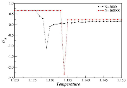
Figure 2 Bindercumulant versus temperature for N=2000 and 160000 sites.

Figure 2 displays the fourth- order Binder cumulant $\left(U_{\text{4}}\right)$ versus temperature. We find that there is a crossing point and the $\left(U_{\text{4}}\right)$  shows a negative dip for the system sizes (N=2000 and 160000 sites). These are typical indications of a first-order phase transition.¹³ To confirm whether a first-order transition is really taking place, we also plot the distribution of the magnetization very close to $T_c$  (Figure 3). Here, we calculate $T_c$ as being the temperature where the peak of the specific heat is maximum $\left(C_{max}\right)$ (Figure 4). Here, we found out T_c1.133(2).

Figure 3 PDF of for $\left|m\right|$ q=3 and N=160000 sites. The double peak in the magnetization distribution indicates that the transition is of the first-order.

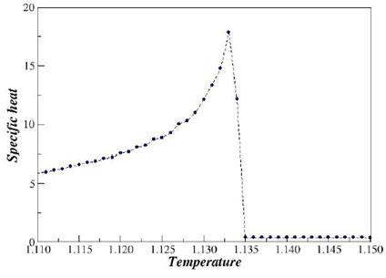
Figure 4 Plot of the Specific heat versus temperature for N=1600000 sites. Here, T_c1.133(2).

As depicted in Figure 3, we show the probability density function (PDF) of the order parameter. From this PDF, one can see that the phase transition is discontinuous or first-order for q=3 and N=160000 sites. In the Figure 4, we plot the specific heat versus temperature for N=160000 sites. In the Figure 5, we show the Binder parameter minima versus temperature and again the first-order phase transition is verified. The critical temperature estimate for the largest N is T_c1.133(3), that is identical to $T_c$ of the specific heat.

Figure 5 Plot of the energetic Binder versus temperature N=160000 sites T_c1.133(3).

In the present work, we have shown that, by considering the three-states ferromagnetic Potts model on Solomon networks there is a phase trasition. Different from the Potts model with q=3 on square lattice that presents a second-order phase transition, here, we show that this same model on Solomon networks presents a first-order phase transition. Therefore, our results agree with the Harris-Luck criterion for Solomon networks.

The author would like to thank the Brazilian agencies CNPq and Capes.

The author states that there is no conflict of interest.

1. Malarz K. Social phase transition in Solomon network. International Journal of Modern Physics C. 2003;14(5):561–565.
2. Erez T, Hohnisch M, Solomon S. Economics: Complex Windows. Germany. Springer; 2005:201–217.
3. Goldenberg J, Shavitt Y, Shir E, et al. Distributive immunization of networks against viruses using the ‘honey–pot’ architecture. Nature Physics. 2005;1:184–188.
4. Herrero CP. Ising model in small–world networks. Physical Review E. 2002;65(3):066110.
5. Pekalski A. Ising model on a small world network. Physical Review E. 2001;64(5):057104.
6. Landau DP, Binder K. A Guide to Monte Carlo Simulations in Statistical Physics. 2nd ed. UK: Cambridge University Press; 2005.
7. Silva PROD, Lima FWS, Filho NRC. Potts model with q=3 and 4 states on directed small–world network. Computer Physics Communications. 2003;184(12):2746–2750.
8. Lima FWS. Potts Model With q=3 on Directed Erdös–Rènyi Random Graphs. Physics & Astronomy International Journal. 2017;1(6):00040.
9. Erdös P, Rényí A. On the evolution of random graphs. Publication of the Mathematical Institute of the Hungarian Academy of Sciences. 1960;5:17–61.
10. L'Ecuyer P. Efficient and portable combined random number generators. Communications of the ACM. 1988;31(6):742–751.
11. Janke W, Villanova R. Two–dimensional eight–state Potts model on random lattices: A Monte Carlo study. Physics Letters A. 1995;209(3–4):179–183.
12. Binder K. Theory of first–order phase transitions. Reports on Progress in Physics. 1987;50(7).
13. Binder K, Herrmann DJ. Monte–Carlo Simulation in Statistical Physics. In: Fulde P, editor. Germany: Springer; 1988:61–62.