In this brief review, the evolution of Thermal-unit Growth Coefficient (TGC) is presented, from the initial model adapted to gilthead sea bream, until the Quantile TGC-Mixed Model. The two first adaptations were the effective temperature, and the quantile regression, that allowed the possibility of describing the evolution of weight distribution along the production cycle. The second adaptations consisted in considering the temperature seasonal curve and integrating the two growth exponents (1/3 and 2/3) in a mixed model. The final Quantile TGC-Mixed Model is a very interesting tool for evaluating production strategies in gilthead seabream and optimizing its economic profit, but each fish farm should have its own model in basis historical data.

Keywords: Modelling fish growth, Quantile regression, Growth in marine cages, Thermal Growth Coefficient (TGC), Fish farm management

Gilthead sea bream (Sparus aurata L) and European sea bass (Dicentrarchus labrax L) are produced in the Mediterranean Sea, mainly in Turkey, Greece, Spain, Egypt and Italy, 85% of global production, around 315 thousand tons in 2014. Economic value was 1.962 million USD (JRC, 2016) being an important economic activity in coastal zones.

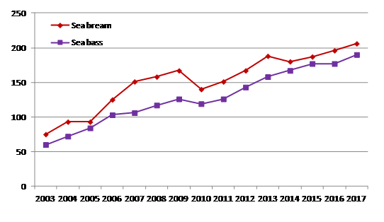
Both species are grown mainly in marine cages, although a minimum production is located in extensive ponds and also in tanks, mostly for juveniles. The evolution of production of both species shows a steady increase from 2003 to 2016 (Figure 1), with some falls in several years as a consequence of the global crisis.

Figure 1 Evolution of Mediterranean production (thousand tons) of gilthead sea bream and European sea bass (Source: APROMAR).

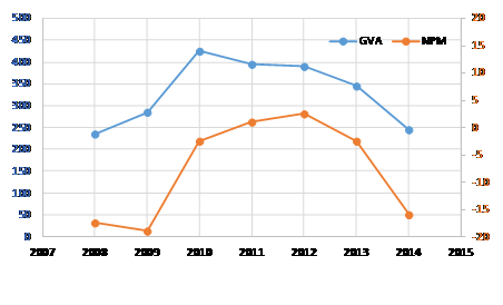
Economic data are only available within EU countries, which mean around the 50% of total Mediterranean `production, with 149 thousand tons and 1009 million USD (JRC, 2016). Gross Value Added (GVA) was positive in the whole period 2009-2013, but negative in 2014, moreover Net Profit Margin (NPM) was negative in all period except in 2011 and 2012 (Figure 2). This situation is partially due to low sales price of both species, around 6.36 USD/kg, because in most cases total operating costs are higher than total income (JRC, 2016). Nevertheless, price is difficult for farmers to control, so the other possibility to improve profit would be to reduce operative costs through an improvement of management of biomass stock and feeding.

Figure 2 Evolution of Gross Value Added (GVA) (thousand USD) an Net Profit Margin (NPM) (%) of gilthead sea bream and European sea bass (Source: JCR).

Currently, feeding systems in marine cages are based in the “daily feeding rate”, which requires to know the water temperature, the total weight of fish inside the cage, and average weight of fish. Temperature is easily measured every day, fish weight is estimated periodically (2-3 months) using several systems (manual weighting or visual sounds), and total weight is calculated in function of the number of fish, which is complicate due to the escapes, the effect of predators and the mortality.

Direct estimation of total weight inside the cages is a complicated task, but some advances have been made using ultra-sounds. Daily knowledge of fish biomass would allow farmers to feed the fish in an optimum way, but this is currently impossible, this is why the feeding management in cages consist in improving the accuracy of fish quantity estimation, and using growth models to estimate the evolution of fish weight between two samples. The inconvenient of this is that fish farms generally use standard growth models, which must be adapted to each farm, and even to each cage, for an optimum feeding strategy.

Moreover, several management operations in marine cages, such as sieving and splitting of batches, prevision of sales and planning of harvesting, require a prediction of fish weight several months before hand, that is why it is necessary to relay on an accurate growth model adapted to the real conditions in each farm. Finally, when it come to planning new fish farms, it is highly convenient to know the growth of fish in their regional location, which requires to have a good growth model.

In the early past century, Von Bertalanfy developed his well known growth model, often used for describing natural population growth in all age classes, but not useful in aquaculture, provided that fish only belongs to 0+ or 1+ class.

Specific Growth Rate (SGR) has been used many years to describe growth in aquaculture (Equation 1), but it is not a good model for making predictions at medium or long term. Plus, SGR model does not consider water temperature, and fish growth is very temperature dependent, mainly in sites with a wide oscillation, as in the Mediterranean Sea where temperature range between 12 and 26 ºC.

$SGR=\frac{\ln (W_f)-\ln (W_i)}{t}$

$W_f=W_i\times \exp (SGR\times t)$   (Eq. 1)

Because of this, several exponential models considering temperature (Equation 2) were developed by Lupatsch et al.^1-3

$WG=a\times W_i{}^b\times \exp (c\times T)$   (Eq. 2)

Finally, a new Thermal-unit Growth Coefficient (TGC) model based in the sum of daily temperature (Equation 3) was reported by Cho & Bureau⁴ or salmonids, and adapted by Mayer et al.⁵ in gilthead sea bream using the effective temperature (> 12ºC).

$TGC=\frac{W_f^{\frac{1}{3}}-W_i^{\frac{1}{3}}}{{\displaystyle \sum Tef}}$   (Eq. 3)

One of the advantages of TGC model is than its value is independent of fish weight, making it possible to solve the final weight (Wf) in function of initial weight (Wi) by forecasting the sum of temperature in the next period (Equation 4).

$W_f={\left(W_i^{\frac{1}{3}}+TGC\times \sum Tef\right)}^3$   (Eq. 4)

Nevertheless, Dumas et al.⁴ reported three TGC values exits in trout for three weight stanzas (< 20 g, 20-500 g and > 500g). Likewise, Mayer, Estruch and Jover made a change in gilthead sea bream TGC model, due to the fact that for a weight lower than 117 g TGC responds better to a 1/3 exponent, and for a weight over 117 g TGC responds to a 2/3 exponent, the authors named it the Mixed TGC model and included a sinusoidal temperature curve (Equation 5) in the growth model to simulate the seasonal TGC growth.

$W(t)=\left(W_0^b+TG{C}_b\cdot \left(\left(T_m-12\right)\cdot \left(t-t_0\right)-T_D\frac{365}{2\pi }\left(\cos \left(\frac{2\pi \left(t-\alpha \right)}{365}\right)-\cos \left(\frac{2\pi \left(t_0-\alpha \right)}{365}\right)\right)\right)\right)\frac{1}{{}^b}$   (Eq. 5)

A very good revision of growth models has been recently published by Seginer,⁹ including the effect of temperature and feed ration.

Traditionally, fish growth models have only considered the average fish weight, but taking into account that the variability in a cage with 200 thousand fish can be very high, the optimum management requires more information about weight distribution. Because of this, Mayer et al.⁷ applied the quantile regression to TGC model to determine the dispersion of fish weight along production cycle (Figure 1).

Estruch et al.² have recently showed the potential of Quantile Mixed TGC model as a new tool for improving management in fish farms. For example, to decide the optimum time for harvesting a cage (300 thousand fish and 85% survival), a simulation of total final weight, duration of cycle and sale price of harvest was made for quantiles 0.25, 0.50 and 0.75 reaching 400, 500 and 600 g weight (Figure 2). Duration of growth, total fish harvested and value of sale increased with fish weight in each quantile. The manager of each fish farm must choose the best alternative in function of operation cost and sale planning, but the decision will be based in its own growth model (Figure 3-4).

Figure 3 Gilthead sea bream quantile growth curves considering three levels of growth (low, medium and high (Simulation available in www.cursodeacuicultura.upv.es/estruch.html).

Figure 4 Estimation of a) production cycle duration (days), b) total weight harvested (tons) and c) sales values (thousand USD) of gilthead sea bream corresponding to when the quantiles 0.25, 0.50 and 0.75 reach the weights 400, 500 and 600 g.

Growth models for fish are a fundamental tool for managing marine cages (fish stock, feeding, harvest and sales, etc), in fact, most of commercial software for fish farms include a general model that must be manually adapted to each marine installation, but the result is not optimum and it could be improved to provide better economic results.

A proposal for the future is to establish a particular Quantile Mixed TGC model for each fish farm, developed in function of historical growth data and temperature and considering other local characteristic such as water quality, marine currents, stock management, etc, even though in reality the best solution would be to have several model for different origin of fish, type of feed and feeding estrategy, etc.

Moreover, considering that growth of fish can vary each year in function of quality of juveniles, the growth model in every farm must be adapted in each cage depending on first weight samples, but this matter is still under development.

None.

The authors report no conflicts of interest.

1. Lupatsch I, Kissil GW Predicting aquaculture waste from gilthead seabream (Sparus aurata) culture using an nutritional approach. Aquat Living Resour. 1998;11(4):265–268.
2. Lupatsch I, Kissil GW, Sklan D  Defining energy and protein requirements of gilthead seabream (Sparus aurata) to optimize feeds and feeding regimes. The Israeli Journal of Aquaculture. 1998;55(4):243–257.
3. Mayer P, Estruch VD, Blasco J, Jover M Predicting growth of gilthead sea bream (Sparus aurata) in marine farms under real productions conditions using temperature and time–dependent models. Aquaculture Research. 2008;39(10):1046–1052.
4. Dumas A, France J, Bureau D. Evidence of three growth stanzas in rainbow trout (Oncorhinchus mykiss) across life stages and adaptation of the thermal–unit growth coefficient, Aquaculture. 2007;267(1–4):139–146.
5. Estruch VD, Mayer P, Roig B, et al. Developing a new tool based on a regression mixed model for optimizing gilthead sea bream (Sparus aurata) farm management. Aquaculture Research. 2016;pp.1–12.
6. Joint Research Center. Economic Report of EU aquaculture sector (STECF–16–19). European Commission. 2016
7. Mayer P, Estruch VD, Martí P, et al. Use of quantile regression and discriminant analysis to describe growth patterns in farmed gilthead sea bream (Sparus aurata). Aquaculture. 2009;292(1–2):30–36.
8. Mayer P, Estruch VD, Jover M. A two–stage growth model for gilthead sea bream (Sparus aurata) based on the thermal growth coefficient. Aquaculture. 2012;358–359:6–13.
9. Seginer I. Growth model of gilthead sea bream (Sparus aurata) for aquaculture: A review. Aquacultural Engineering. 2016;7015–32.