Efficiency of mixing, resulting from the reflection of an oscillatory internal wave field off a continental slope is investigated using a linear approximation. The continental slope is modelled with a corrugation running down a slope. Efficiency of deep ocean mixing is associated with the energy of the flow radiating into an interior of the ocean due to interaction with the corrugated slope. The effects of the corrugation geometry and the earth's rotation on resulting energy is analyzed analytically in the vicinity of the critical values of the slope.

The Atlantic Ocean's deep canyons are home to a diversity of marine life, including corals and other species that attach themselves to rocky ledges.^1,2 The configuration of the eastern and western sides of the Atlantic Ocean strongly influences the movement of internal ocean's currents.³ and, ultimately, the nature of the deep-sea biota. Strong bottom flows, sometimes reaching storm proportions, cause a strong mixing processes playing an important role in redistributing sediments and organic matter in deep water, leading to the formation of vast sediment drifts.⁴ Waves produced at the sea floor propagate into the ocean interior, generating small-scale mixing processes that affect circulation, heat transport, and nutrient distribution and, in turn, biological productivity. Observations by Polzin KL.⁵ based on measurements of microstructure show that mixing is considerably increased over bottom irregularities. In particular, tidal flows result in mixing directly above the boundaries, in which case an issue of particular importance is the rate at which oceanic fluid from the interior is exchanged with fluid at the sloping boundary. According to Armi L.¹ this exchange plays a paramount role in the efficiency of boundary mixing, allowing it to contribute significantly to the global overturning circulation.^6–8 Current estimates suggest that 40-50% of the energy required for a deep-ocean mixing is injected by tide-topography interactions with the remainder coming from wind forcing.^9,10 Stratified flows over topography are of interest for meteorology as well.^11,12

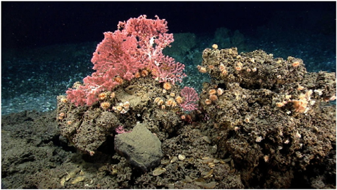
The total length of the world's continental slopes sums up to 300,000 km. More than one-half of all continental slopes descend in deep sea trenches. The rest of the slopes descend into the shallow marine sediments (Figure 1). It has been observed that the "Pacific Continental Slope" is steeper than the "Atlantic Continental Slope" whereas the continental slope gradients are flattest in the Indian Ocean.¹³ The continental slopes occupy almost 8.8% of the world's surface. Geological forces formed the Mid-Atlantic's deep submarine canyons over millennia. The peaks of these canyons today lie near what was the paleo-shoreline, where ancient river channels once flowed into the ocean when global temperatures and sea levels were lower. Eventually temperatures warmed, sea levels rose, and the ocean reached the modern shoreline.¹⁴ Canyons in the U.S. East Coast were a high priority for federal and state agencies tasked with research and management responsibilities, particularly because of deep-sea corals. As has been pointed out in.¹⁵ the role of deep see corals as possible habitats for fishes has only recently been addressed. Some findings suggest that increased habitat heterogeneity in canyons is responsible for enhancing benthic biodiversity and creating biomass hotspots.¹⁵ Figure 2 is used to illustrate cup corals and bubblegum corals that were found on hard substrate near the edge of a mussel bed while exploring a gas seep area near the northeast submarine canyons. Even with increased research activities in recent years, the effects of mixing process at the bottom irregularities and their effects on a wide variety of habitats remain poorly known.^15–17

Figure 1 Upper panel: 3D-image over the continental shelf outside Senja/Andoya. Data from Kartverket and MAREANO. Acvailable at https://www.ngu.no/en/topic/continental-shelf-and-slopeSchemtic
Lower panel: Canyons on the edge of the Continental Shelf show former river channels of Pliocene/Pleistocene age. Source: National Oceanic and Atmospheric Administration (NOAA), Deep-Water Mid-Atlantic Canyons Exploration 2011.

Figure 2 Cup corals and bubblegum corals that were found on hard substrate near the edge of a mussel bed while exploring a gas seep area near the northeast submarine canyons. Image courtesy of 2013 Northeast U.S. Canyons Expedition, also available at http://oceanexplorer.noaa.gov/ explorations/ 16carolina/ background/ submarine-canyons/ submarine-canyons.html.

The primary focus of this article is to analyze the efficiency of mixing process that results from a reflection of an oscillatory background internal wave field off the corrugated continental slope. The corrugation is assumed to be running directly up and down the slope. Efficiency of mixing is associated with the energy radiating into interior of the ocean of the corrugated slope. We focus on the case when the topography produces only a small perturbation to the flow field. The presence of the topography generates a localized disturbance, which propagates into the ocean interior from the source region in the form of an internal gravity wave field. This work aims to provide a better understanding of the effects of the corrugation geometry and the earth's rotation on the resulting energy radiation in the vicinity of the slope.

In the ocean, time dependent tidal currents passing over topographic bottom features are a significant source of internal waves.^18–22 In our model, the ocean is idealized as vertically unbounded medium and, since the source of the wave energy is at the bottom, all waves have upward group velocity and the radiated energy freely escapes to $z=+\infty$ . In this work we investigate the efficiency of mixing due to time dependent harmonic basic flow of the form $\overrightarrow{u_0}(t)=(U_0\cos (w_{0}t), V_0\sin (w_{0}t), W_0\sin (w_{0}t))$ .Our model is includes Coriolis effects. Although the presence of an oceanic free surface is also significant.²³ perhaps more so than rotation, we note that if we assume that waves generated by the topography are dissipated before returning to the bottom after reflection from the free surface, our solution will be of physical reference to the real ocean see e.g.,.⁶ where reduced mixing efficiency arising from boundary-layer physics is actually claimed.^24.–26

A simple linear solution for flow at constant velocity and constant stratification over a Witch of Agnesi-shaped mountain of height H and half-width $L:h(x)=H{L}^2/(L^2+x^2)$  (in our model, we consider the same form of corrugation) has been investigated in.²⁷ The current knowledge of flows over hills is summarized in.^28–30 and.¹⁹ The tides have been reexamined in.³¹ as a possible source of energy for diapycnal mixing in the ocean interior. Evidence from satellite altimetry indicates that as much as 30% of tidal dissipation occurs in the open ocean.³² a process previously thought to occur almost exclusively on the continental shelf. Much recent activity has therefore been focused on understanding where and how this open ocean component of tidal dissipation occurs.^{5,13,23,29,33–34} Previous studies of internal wave generation by flow over topography have identified two important controlling parameters see e.g..^13,36 The first parameter $\epsilon =|\nabla H|/s$  is a measure of the relative steepness of the topography, where the bottom is at $z=-H+h(x,y)$  with H being the depth, and

$s=\frac{k}{m}=|{(\frac{w^2-f^2}{N^2-w^2})}^{\frac{1}{2}}$   (1)

is the slope of an internal wave group velocity characteristic. Here we use customary notation (see e.g.³⁷ in which k is the horizontal wavenumber, m is the vertical wavenumber, ω is internal wave frequency, f is the Coriolis frequency, and N is the buoyancy frequency. As has been pointed in.¹³ it is most likely that the most efficient mixing is resulting from the reflection of an internal wave from a slope at values α close to its critical angles α^c for which tan α^c given by (1). The second parameter is $RL=U0/(L\omega 0)$  where L is topographic length scale. This parameter is a ratio between the tidal excursion distance $U_0/w_0$  and the length of the topographic feature. It is one measure of nonlinearity. A third parameter is $\alpha /H$  where αis the topographic amplitude and H is the water depth away from topography.

Bell.³³ considered the process of internal gravity wave generation by simple harmonic flow $u0=U0\cos (\omega 0t)$ of a stratified flow over an obstacle. His analysis was for an infinitely deep ocean with thee-dimensional topography h(x,y) in the limit $\epsilon <<1,$  with finite $R_L$  see e.g..^13,36 Bell's model linearizes the problem by applying the boundary condition at z = 0, as we do here in a rotated three-dimensional coordinate system, rather than at the bottom topography $z=-H+h(x)$  (we show later that , in an appropriately rotated coordinate system, we can linearize the problem about z = 0 as in Bell paper although, originally, the bottom is at $z=\alpha y$ ). Balmforth et al.³⁸ have extended Bell's theory to steeper topography $(0<\epsilon <1)$ but their linearization is justified provided that $R_L<<1,$ i.e., the tidal excursion is much less that the scale of the topography. Khatiwala.²³ in part based on Bell.³³ examines the problem of internal wave generation by the interaction of an oscillating tidal flow with two-dimensional bottom topography $z=-H+h(x)$ z. Unlike Bell's theory, which is applicable for a fluid of infinite depth in which energy input at the bottom radiates upward, Khatiwala imposes an upper rigid lid boundary condition resulting in a horizontal energy flux. Thorpe.^39,40 extended the wave generation problem to uniform flow along a corrugated slope. His solution includes the effects of the earth's rotation and he considered corrugations that are at an angle to the direction of steepest slope. MacReady 4 Pawlak.⁴¹ presented an alternative derivation of Thorpe's solution (neglecting the effect of rotation) and extended it to flows above and below the low speed cutoff. Legg.¹³ performed numerical experiments for internal tide generation for a continental slope characterized by ridges and valleys running up and down the slope. Other related studies by Kunze.⁴² and Nash & Mourn.^43. have considered internal tides on the continental slope and internal hydraulic flows on the continental shelf , and their results are not directly applicable to the deep ocean processes considered here. The process of generation of internal waves due to tide/topography interactions associated with oscillating along-isobath currents impinging on a ridge running down a slope with an inclusion of large tidal excursion to generate harmonics has been considered in Ibragirnov.⁴⁴ The experimental work confirming some of the analytic predictions from.⁴⁴ have been reported recently in.⁴⁵

Here we focus on the corrugation scales and the effects of rotation on the energy flux in the vicinity of the critical slope ${\alpha }_c$ . Additionally, we also analyze the effects of concavity of the corrugation on the resulting energy flux which has not been analyzed in.⁴⁴ Thus this work combines that of.⁴³ for harmonics generated by large tidal excursion over weak topography (small-amplitude $h/H<<1$  gentle subcritical slope $h_x/s<<1$ ) on a flat bottom with recent extensions on a slope.^39,41

Governing equations

For the sake of definiteness, we set the axes as:x^/ (assumed eastward),y^/ (northward) and $\widehat{k}$^/ is the unit vector in the vertical z^/ direction, opposite gravity

is the unit vector in the vertical $z^{\text{'}}$  direction, opposite gravity (see (Figure 3) for the topographic coordinates). The fluid velocity is $\overrightarrow{u}$  = (u, v, w) relative to the Cartesian coordinate system (x',y',z'). Within the Boussinesq approximation, the governing equations of motion for internal waves, observed in a system of coordinates rotating with angular velocity $\overrightarrow{\Omega }$  are written in the vector form as follows (see e.g.²⁸

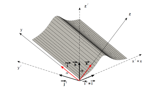
Figure 3 Corrugated slope sketch. To accommodate a sloping ocean floor, the model is considered in the system of coordinates rotated about the x axis by the slope angle a, so that in the new coordinate system the y—axis is directed upslope and z is perpendicular to the slope.

${\rho }_0{}_{\left[\frac{\partial \overrightarrow{u}}{\partial t}+\overrightarrow{u}.\nabla \overrightarrow{u}+2\overrightarrow{\Omega } \times \overrightarrow{u}\right]}{ }_{= -\nabla p-g\rho \widehat{k}/},$   (2)

$\frac{\partial \rho }{\partial t}+\overrightarrow{u}.\nabla \rho +w\frac{d\overline{\rho }}{d{z}^{\prime }} = 0,$   (3)

$\nabla .\overrightarrow{u} = 0,$   (4)

where g is the acceleration due to gravity so that p and ρ are to be interpreted as the pressure and density departures from their mean state

$\overline{\rho }\left(z^{\prime }\right)=-\frac{{\rho }_0}{g}{{\rm N}}^2{z}^{\prime }, \overline{p}\left(z^{\prime }\right)=p_0-{\rho }_{0}g{z}^{\prime } -g{\displaystyle \underset{0}{\overset{z^{\prime }}{\int }}\overline{\rho }\left(\xi \right)} d\xi$   (5)

in which ${\rho }_0$  is the constant reference density, $\overline{\rho }(z\text{'})$ is a background stable density profile with the associated buoyancy frequency N defined by

$N^2=-\frac{g}{{\rho }_0}\frac{d\overline{p}}{d{z}^{\text{'}}}$   (6)

and we require ${\rho }_0+\overline{\rho }$  and $\overline{\rho }$  to be consistent with the state of rest, i.e.

$\frac{d\overline{p}}{d{z}^{\text{'}}}=-({\rho }_0+\overline{p)}g$   (7)

The quantity N, which is assumed to be a constant in the frame of the present study, measures the degree of density stratification of a fluid with average potential density $\overline{\rho }(z)$  and thus represents the frequency with which a vertically displaced fluid element would be expected to oscillate because of restoring buoyancy forces.

The traditional f —plane approximation is made whereby we take $2\overline{\Omega } = (0,0,f),$  where f is the inertial frequency which depends on the rotation rate of the earth (angular velocity $\text{Ω =2π rad/day}\approx \text{0}{\text{.73×10}}^{\text{-4}}{\text{s}}^{\text{-1}}$ ).

The oscillatory three-dimensional time-dependent background flow over a uniform flat slope z = 7y is given by

${\overrightarrow{u}}_0=\left(U_0\cos \left({\omega }_{0}t\right), V_0 \sin ({\omega }_{0}t), \gamma V_0\sin \left({\omega }_{0}t\right)\right)$   (8)

where $\gamma = \tan \alpha ,$  the cross-shelf velocity U₀ is assumed to be constant and w₀ the frequency. Since we are mostly interested in tidal flows, hereafter we consider flows forced at M₂ tidal frequency, $w{M}_2$

${\omega }_0= \omega M_2\sim 1.4 \times {10}^{-4} s^{-1}$   (9)

Thus the oscillating flow (8) is driven by the barotropic tide.

Since waves are generated not only at the fundamental frequency but also at all of its harmonics $w_n=n{w}_0$  less than N, our analysis will include, in general, an infinite number of discrete internal wave modes satisfying the dispersion relationship for internal waves. However, we will be interested only in the radiating part of the solution so that the mode numbers will be limited. Small perturbations are introduced:

${}_{u= u_{0 }+\in \widehat{u}, v=v^{\text{'}}{}_0+ \in \widehat{u}, w={w^{\prime }}_0+\in \widehat{w}, p= \overline{p}+\in \widehat{p}, \widehat{p}= \overline{\rho }+ \in \widehat{p},}$   (10)

where $\in <<1$  is a small parameter.

Formulation of the main result

As has been shown in.⁴⁴ in the system of coordinates that is moving with the background flow $u_0=U_0\cos (w_{0}t)$  and that is rotated about the x-axis by the slope angle α, the result­ing non-dimensional, normalized time average power (energy flux) in the internal wave field, associated with the radiating part of the linearized model for small perturbations introduced by (10), is written as

$\begin{array}{l}\langle \tilde{p}\rangle =\langle p\rangle /\frac{1}{4}\Pi {\rho }_0{U}_0^{2}N{H}^2 \\ = 4{\beta }^2\Sigma {\displaystyle \sum _{n=1}^{n_{\max }}\frac{n^3{\lambda }^3{\left(n^2{\lambda }^2-{\gamma }^2\right)}^{\frac{1}{2}}{\left(1-n^2{\lambda }^2\right)}^{\frac{1}{2}}\left(n^2{\lambda }^2-{\widehat{f}}_d^2\right)}{\left(n^2{\lambda }^2-{\widehat{f}}_d^2\right)n^2+\left(1-n^2{\lambda }^2\right){\widehat{f}}_d^2{\sin }^2\alpha }}\\ {\displaystyle \underset{0}{\overset{\infty }{\int }}\frac{e^{-2\tilde{k}}}{\tilde{k}}{J}_n^2\left(\frac{\sqrt{2}\tilde{k}}{\beta \lambda }\right) d\tilde{k}}\end{array}$   (11)

where the following notation is used:

$\langle p\rangle = \frac{{\omega }_0}{2\pi } {\displaystyle \underset{0}{\overset{2\pi /{\omega }_0}{\int }}\mathrm{Re} \left\{F\left(t\right)\right\}} u_0\left(t\right) dt$   (12)

is the power input into the internal wave field averaged over the fundamental period $2\pi /w_0$  and

$F\left(t\right) = {\displaystyle \underset{-\infty }{\overset{\infty }{\int }}p\left(x,z,t\right)}|z=0 \frac{dh}{dx}dx,$   (13)

is the net force exerted into internal wave field due to the given oscillatory background flow in the vicinity of the bottom topography (see also.³³). Also,

${\widehat{f}}_d^2 = {\sin }^2\alpha + {\gamma }^2{\cos }^2\alpha ,$   (14)

is the notation and $\beta ,\lambda ,\gamma ,\tilde{k}$  and $\widehat{\eta }$ are the following nondimensional parameters:

$\lambda -\frac{{\omega }_0}{{\rm N}}, \gamma =\frac{f}{{\rm N}}, \tilde{k} =kL, \widehat{\eta } =\frac{\widehat{h}}{LH}, \beta =\frac{\sqrt{2}NL}{U_0}$   (15)

in which k is a horizontal wave number, $\widehat{h}(k)$  is the Fourier Transform of the corrugation geometry h(x) that forces the motion, J_n, is the Bessel function of the first kind, and H and L are the horizontal and vertical scales of the corrugation h(x).

Since the generated waves are independent of the upslope coordinate y, the wavevectors must be in x, z plane. Two such vectors exist for sufficiently small α. Thus, as has been justified in.⁴⁴ the radiating waves exist for frequencies $w_n=n{w}_0$ , where

$\left|n\right| \in S_N =\left[n_f,n_N\right]$   (16)

$n_N= \left[\frac{N}{{\omega }_0}\right] , n_f= \left[\frac{\widehat{f}}{{\omega }_0}\right]+ 1,$   (17)

where here.^x means the greatest integer less that or equal to x. In particular, n_N = 7 for $w_n=n{w}_0$ . If $w_n^2 < \widehat{f^2}$ or $w_n^2 > N^2$ the waves are evanescent. As follows from the dispersion relation (1), waves of frequency $w_n$ , lying between f and N can propagate freely only for angles

$\alpha < \arcsin {\left(\frac{n^2{\omega }_0^2-f^2}{N^2-f^2}\right)}^{\frac{1}{2}}$  (18)

which means that α is fixed by some harmonic of the high-frequency wave. This means that waves of frequency $w_n$ , can exist only if the slope angle $\alpha ={\alpha }_{n\theta }$  is such that

${\sigma }_{n,f}={\omega }_n^2-{\widehat{f}}^2>0.$   (19)

As seen from (11), the normalized power $\langle \tilde{p}\rangle$ has a singularity in the in the vicinity of the critical angles $\alpha ={\alpha }_{n\theta }$  i.e. the singularity occurs if

${\alpha }_{n\theta } = {\alpha }_{n\theta }^c= \arcsin {\left(\frac{n^2{\omega }_0^2-f^2}{N^2-f^2}\right)}^{\frac{1}{2}}$   (20)

which is the slope of an internal wave group velocity characteristic that has been identified in the Introduction by Eq. (1).

Remark: Radiating waves of frequency w_n, do exist for angles satisfying the condition (19), so we write a $\alpha ={\alpha }_{n\theta }$ in order to indicate that the value of critical slope ${\alpha }^c$ is individual for each mode number n and latitude θ.

The most efficient mixing occurs in the vicinity of the critical slopes defined by (20), i.e. when a $\alpha > {\alpha }_{n\theta }^c$ . Thus evanescent modes do not contribute to F (t) because of upward radiation of energy. So, mixing occurs for those mode numbers n, that satisfy (16) and those angles $\alpha { }_{n,\theta ,}$ for which (19) holds.

To make some comparison with the Bell's results in.³³ and to analyze the effects of rotation and the topographic scales on the energy flux studied in.⁴⁴ we consider a specific example when the corrugation has the form

$h\left(x\right) = \frac{H}{1+{\left(x/L\right)}^2}.$   (21)

Our model is analyzed for the fixed value of parameters for which (15) yields

$U_0 =1.4 \times {10}^{-3}m{s}^{-1} , N ={10}^{-3}{s}^{-1},$   (22)

$\frac{U_0}{\sqrt{2}} \approx 1, \lambda =\frac{{\omega }_M{}_{{}_2}}{N}= 0.14, \beta \approx L,$   (23)

Since the parameter H does not appear in (11), without loss of generality we can set H = 1.
To analyze the resulting power input $\langle \tilde{p}\rangle$ , we first investigate the convergence of the integral

$Q_n\left(\beta \right) = {\displaystyle \underset{0}{\overset{\infty }{\int }}\frac{e^{-2\tilde{k}}}{\tilde{k}}}{J}_n^2 \left(\frac{\sqrt{2}\tilde{k}}{\beta \lambda }\right) d\tilde{k} = \underset{\in \to \infty }{\lim }{\displaystyle \underset{\in }{\overset{M}{\int }}\frac{e^{-2\tilde{k}}}{\tilde{k}}}{J}_n^2\left(\frac{\sqrt{2}\tilde{k}}{\beta \lambda }\right) d\tilde{k},$   (24)

which is the approximation of the improper integral in (11) for M >> 1. Figure 4 is used to demonstrate the results of numerical simulations of $Q_{n(\beta )}$  versus M at fixed values of ε. In our further simulations we use the values M = 10 and ε = 0.001.

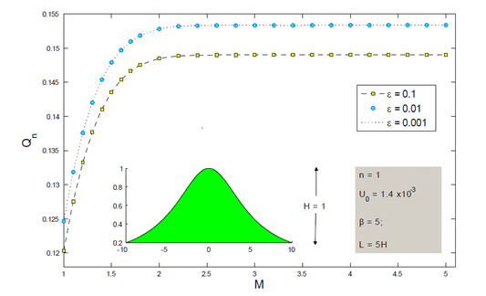
Figure 4 Convergence of the integral $Q_n$   $(\beta )$ as M→∞and ∈→ 0.

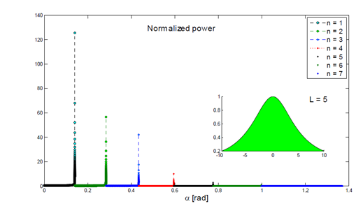
Figure 5 shows the results of numerical simulations for the normalized power (that can also be interpreted as a vertical energy flux) $\langle \tilde{p}\rangle$  without rotational effects as a function of slope ${\alpha }_{n0}$ (i.e. purely equatorial waves as observed at latitude $\theta =0^0$ North) for L = 5H and the fixed values of parameters λ and U₀ given by (22). As we found earlier, the waves are nearly singular at the vicinity of the critical slopes ${\alpha }_{n\theta }^c$  determined by the condition (20), which makes the energy flux increasing rapidly at the vicinity of ${\alpha }_{n\theta }^c$ . This agrees with the suggestion of Legg, .³⁶ about an efficiency of mixing in the deep ocean due to reflection of an internal waves from critical slopes. In particular, because of singular behavior $\langle \tilde{p}\rangle$ near the critical slopes ${\alpha }_{n\theta }^c$ the visualization depends of stepsize of α. We further use the stepsize $\Delta \alpha ={10}^{-6}$ . As we observe from Figure 5, the dominant contribution of energy distribution in internal wave field is due to waves of fundamental frequency with n = 1. We also observe the dramatic energetic drop at slopes of $\alpha >{\alpha }_{n\theta }^c$  but with subsequent "singular" increase at the successive critical slopes ${\alpha }_{n\theta }^c$ , n > 1.

Figure 5 Vertical energy flux $\langle \tilde{p}\rangle$  as a function of slope a at latitude 0 deg North for L = 5 and stepsize $△\alpha ={10}^{-6}$ .

The effects of the topographic horizontal scale L on the normalized power $\langle \tilde{p}\rangle$  of the fundamental frequency n = 1 is demonstrated on Figure 6 in which the normalized power is evaluated at latitude $\theta =0^0$ North (not affected by rotation). Additionally, Figure 6 shows that $\langle \tilde{p}\rangle =\langle \widetilde{{}_{p_{10}}}\rangle$  for the same values of other parameters as been used in Figure 5. As we can see from the numerical simulations presented in this figure, as L goes from 1 to 50, energy monotonically decreases. However, the energy drop is not significant.

Figure 6 First mode normalized power at latitude 0 = 0° North as a function of the characteristic horizontal scale L of the corrugation in the vicinity of α =${\alpha }_{10}^C$

The effects of the topographic horizontal scale on the normalized power $\langle {\tilde{p}}_{no}\rangle$ for all admissible harmonics without rotation (i.e. n ε.^{1, 7}, $\theta =0^0$ North) is also demonstrated on Figure 7 which illustrates the qualitative behavior of _{$\langle {\tilde{p}}_{no}\rangle$}  versus slope α. For better visualization purposes, we use the "fill" option, set ε= 0 and use a larger stepsize $\Delta \alpha ={10}^{-4}$ . As we observe , the higher harmonic waves gradually die off from the wave field for larger values of L. We also remark that, although the maximum values of the normalized power $\langle {\tilde{p}}_{no}\rangle$ look the same for smaller and larger values of L, in actuality it is not quite true; similarly to the observations made in Figure 6 for n = 1, there is an insignificant drop of energy for all admissible modes n.

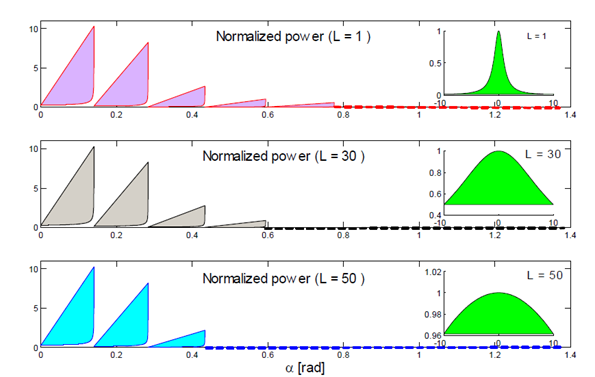
Figure 7 Qualitative energy analysis as a function of slope α at latitude 0 deg North with ε=0 and step size $\Delta \alpha ={10}^{-4}$ .

Figure 8 is used to show the results of numerical simulations for the normalized power $\langle {\tilde{p}}_{n10}\rangle$  versus α for all admissible modes n at latitude $\theta =0^0$ North for L = 1. For better visualization purposes, again we use the "fill" option, set ε = 10^–5 and use the stepsize $\Delta \alpha ={10}^{-6}$ . The more detailed behavior of the first-mode energy in the vicinity of the critical slope ${\alpha }_{n10}^c$  is shown inside the same figure. As Figure 8 shows, the energy attains its maximum not exactly at ${\alpha }_{1,10}^c$  but at some value ${\alpha }_1^{*}$  such that ${\alpha }_1^{\max }<{\alpha }_1^{*}\approx {\alpha }_{1,10}^c$ . Because of singularity, we cannot evaluate the energy at the critical slope ${\alpha }_{1,10}^c$  itself, so we associate the critical slope, say ${\alpha }_1^{*}$ ctrl, which is reasonably close to ${\alpha }_{1,10}^c$ .

Figure 8 Eenergy flux at latitude θ = 10° North with L = H. Here we set ε = 10^-5 and stepsize $\Delta \alpha ={10}^{-6}$ .

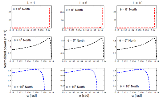
Next, we investigate in more details the effects of rotation and the concavity of the topog­raphy on the resulting energy flux at the vicinity of the critical slopes ${\alpha }_{n,\theta }^c$ . Figure 9 is used to present the results of numerical simulations describing the behavior of the first-mode normalized power $\langle {\tilde{p}}_{10}\rangle$ versus for different values of latitude θ at the vicinity of ${\alpha }_{n,\theta }^c$ . We can see from these plots, that for the given value of θ, changing of the horizontal scale L does not affect appreciably the power $\langle {\tilde{p}}_{10}\rangle$ .However, for the fixed value of L, changes in latitude, have a noticeable impact on the power; not only on the numerical value at the vicinity of the critical slope ${\alpha }_{n,\theta }^c$ , but also on the concavity of the curve, that describes the power. Similarly to the results shown in the detailed plot of Figure 8, we observe here that the energy attains its max­imum not at the critical value of the slope but at some value ${\alpha }_1^{\max }<{\alpha }_1^{*}\approx {\alpha }_{1,\theta }^c$ . For example, when L = 5, we find that: at θ = 5^°, the critical slope is approximated by ${\alpha }_1^{*}\approx 0.1399$ whereas the energy attains its maximum at ${\alpha }_1^{\max }\approx 0.1399$  so that the difference between these two points is not zero and can be approximated by $\Delta {\alpha }^{*,\max }\approx 6.10\times {10}^{-4}$ . Similarly, at latitudeθ = 10^°, we find ${\alpha }_1^{*}=0.1382$ and ${\alpha }_1^{\max }=0.1358$ so that $\Delta {\alpha }^{*,\max }\approx 2.4\times {10}^{-3}$ .

Figure 9 Analysis of the points of energy maximum ${\alpha }_1^{\max }$  and the approximation of the critical slope (i.e. the first zero${\alpha }_1^{*}$ ) for the first-mode of the normalized power at different values of L and latitude.

Figure 10 shows (here, again, we use the "fill" option) the normalized power $\langle {\tilde{p}}_{n\theta }\rangle$ versus a for different values of latitude θ and different values of the horizontal topographic scale L. In particular, we use L = H (upper panel) and L = 50H (lower panel). As has been demonstrated earlier in Figure 7, we observe the gradual disappearance (dying off) of higher harmonic waves for larger values of L. In addition to the "dying off" phenomena, we observe that rotation tends to decrease the overall amount of radiating energy. So, we conclude that increasing the both latitude θ and the horizontal scale L lead to the decrease of the mixing efficiency and removing the higher harmonics waves from the radiating internal wave field. Here we set $\epsilon ={10}^{-3}$  and stepsize $\Delta \alpha ={10}^{-4}$ .

Figure 10 Effect of rotation on the energy flux at different values of the horizontal corrugation scale L

As an illustration to the latter conclusion about the effects of rotation, Figure 11 shows the overall behavior of the normalized power versus a at fixed horizontal scale L = 5H and different values of latitude. In this particular example, shown in Figure 11, the normalized power at latitude θ = 10° North is plotted by red dashed line and the power at latitude θ= 40^° North is plotted by a black pointed line. Here we set ε = 0 and stepsize $\Delta \alpha ={10}^6$ . Finally, Figure 12 is used to visualize the effects of rotation on the resulting first-mode energy flux versus α for different values of latitude and the fixed horizontal topographic scale L = 5H at the vicinity of the critical slopes ${\alpha }_{1,\theta }^c$ . It is similar to the plot shown in Figure 9 but with the larger latitude range. We can see from this list of plots, that the concavity of the curve, that describes the power, is more affected at smaller latitudes, somewhat in the range $\theta \epsilon \left[0^0,{10}^0\right]$ North but for larger values of latitudes, the concavity of the curve is not changed. Here we set ε= 0 and stepsize $\Delta \alpha ={10}^{-6}$ . For example, in panel (b) we find: ${\alpha }_1^{*}=0.138$  and ${\alpha }_1^{\max }=0.1358$ so that $\Delta {\alpha }^{*,\max }\approx 2.2\times {10}^{-3}$ . In panel (c) we find: ${\alpha }_1^{*}$ = 0.1046 and ${\alpha }_1^{\max }$  = 0.047 so that $\Delta {\alpha }^{*,\max }\approx 5.7\times {10}^{-2}$ .

Figure 11 Comparison of the normalized energy flux at latitude θ = 10° North (red dashed line) with the flux at latitude 0 = 40⁰ North (close to critical latitude, plotted by a black pointed line) at the fixed value of L = 5.

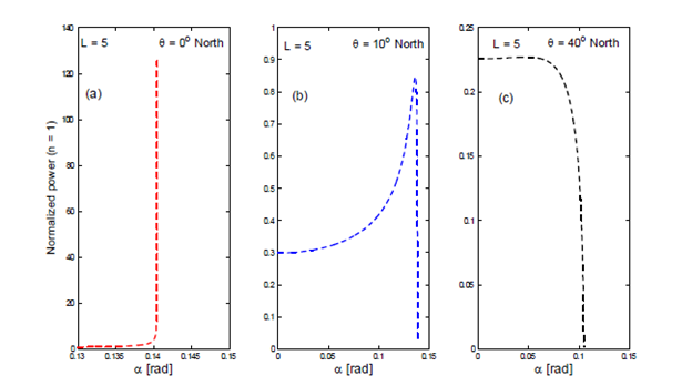
Figure 12 Analysis of the points of maximum ${\alpha }_1^{\max }$  and the first zero ${\alpha }_1^{*}$  for the first-mode of the normalized power at different values of latitude and fixed value of L = 5.

We have investigated the effects of the Earth's rotation and the scales of the given corrugation profile h (x) on the efficiency of mixing associated with the radiating internal wave field that results from the reflection of an oscillatory background flow off a three-dimensional bottom topography, which is used to model a continental slope as shown in Figure 14. The continental slope is modelled by a corrugation given by h (x) running up and down the slope, which is shown schematically in Figure 13. It is shown that the most efficient mixing occurs in the vicinity of the critical slope given by

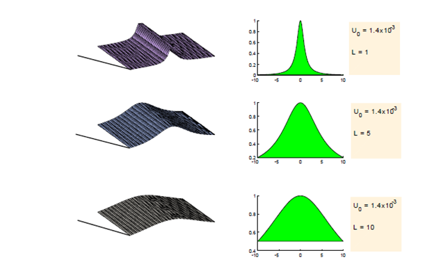
Figure 13 Schematic showing different horizontal scales L of the corrugation geometry.

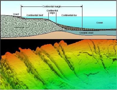
Figure 14 Upper panel: Schemtic presentation of a continental slope representing the submerged border gradually decreasing to the ocean bottom.
Lower panel: Bird's-eye view of continental slope and rise near Hudson Canyon. Note the landslide head-scarps and lobate deposits along the rise. Image source: NGDC.

$\alpha \approx {\alpha }_{n\theta }^c= \arcsin {\left(\frac{n^2{\omega }_0^2-f^2}{N^2-f^2}\right)}^{\frac{1}{2}}$   (25)

which is in agreement with the suggestion of Legg,.³⁶ However, more detailed analysis shows that the radiating part of the energy attains its maximum not at the critical value of the slope but at some value ${\alpha }_1^{\max }<{\alpha }_1^{*}\approx {\alpha }_{1,\theta }^c$ . This fact has not been remarked in Legg.³⁶ and has passed unnoticed in the previous studies in.⁴⁴

It is also found that an increasing in the both latitude and the topographic horizontal L leads to the decreasing in the energy flux, particularly, we observed the gradual dying off higher harmonic waves for larger values of L. This means, that increasing the horizontal scale L leads to the decreasing of the value of the slope ${\alpha }_{n\theta }$ beyond which waves of tidal frequency are not generated. In addition to the "dying off" phenomena, we observe that rotation tends to decrease the overall amount of radiating energy.

We believe that, from physical point of view, the observed "dying off phenomena can be explained by means of the previous relevant results in MacCready 4 Pawlak.⁴¹ according to which, for the values of slope α exceeding the critical value, the fluid parcels do not have enough energy to go over the topography so that the fluid currents are trying to go around the topography.

The interest to this work has been motivated by the increasing interest of oceanographic community to the overpowering amount of untapped energy that is contained in the ocean, and especially in its coastal regions having a complex bathymetry, particularly the prominent corrugations, of the continental margin. It is well recognized that ecosystems are defined by a complex suite of interactions among organisms and also between organisms and their physical environment; a disturbance to any part may lead to cascading effects throughout the system. Ocean mixing has an impact on marine ecosystems through a variety of pathways. Some of the most convincing evidence that a deep ocean mixing affects marine ecosystems comes from studying of effects of warming water on coral reefs. Coral reef ecosystems are defined by the large, wave-resistant calcium carbonate structures, or reefs, that are built by reef calcifiers. The structures they build provide food and shelter for a wide variety of marine organisms. Additionally, it is now recognized that the ocean can produce two main types of alternative energy thermal energy from the sun's heat, and mechanical energy from the tides and waves.^47,48 However, we are unaware of any theoretical, numerical or commercialized projects related to the available alternative energy due to internal waves in the coastal areas of the ocean.

This research was supported in part by the Undergraduate Research Apprenticeship Program (URAP) provided in Spring, 2017 by the Dean's Office - College of Natural and Health Sciences, University of Wisconsin-Parkside.

None.

1. Armi L. Effects of variation in eddy diffusivity on property distributions in the oceans. J Mar Res. 1997;37:515–530.
2. Needler GT. Dispersion in the ocean by physical, geochemical and biological processes. Phil Trans R Soc London A. 1986;319(1514):177–187.
3. Longhurst AR. Ecological Geography of the Oceans, Academic Press, USA, 1998;pp. 398.
4. Hillister CD, McCave IN. Sedimentation under deep–sea storms. Nature. 1984;309:220–225.
5. Polzin KL, Toole JM, Ledwell JR. Spatial variability of turbulent mixing in the abyssal ocean, Science. 1997;276(5309):93–96.
6. Garrett C, MacCready P, Rhines PB. Boundary mixing and arrested Ekman layers: Rotating, stratified flow near a sloping boundary. Annu Rev Fluid Mech. 1993;25:291–323.
7. Ibragimov RN, Vatchev V. Approximation of the Garrett–Munk internal wave spectrum. Phys Let A. 2011;376: 94–101.
8. Ibragimov RN, Jefferson G, Carminati J. Invariant and approximately invariant solutions of non–linear internal gravity waves forming a column of stratified fluid affected the Earth's rotation. Int J Non–Linear Mech. 2013;51:28–44.
9. Ibragimov RN. Nonlinear viscous fluid patterns in a thin rotating spherical domain and applications. Phys Fluids, 2011;23: 123102.
10. Appenzeller CH, Davies CH, Norton WA. Fragmentation of stratospheric intrusions. J Geophys Res. 1996;101:1435–1456.
11. Scorer RS. Environmental Aerodynamics, Halsted Press, USA,1978.
12. Nappo CJ. An introduction to atmospheric gravity waves, Academic Press, USA,2002.
13. Legg S. Internal tides generated on a corrugated continental slope. Part 2: Along–slope barotropic forcing. J Phys Oceanogr. 2004;34(8):1824–1838.
14. Obelcz J, Brothers DS, Chaytor JD, et al. Geomorphic characterization of four shelf–sourced submarine canyons along the U.S. Mid–Atlantic continental margin, Deep–Sea Research II. 2014;104:106–119.
15. Nizinski M, Exploring Carolina Canyons: Submarine Canyons: Discovering         Diversity                in the Deep, Ocean Explorer.
16. Packer DBD, Boelke V, Guida, McGee L.–A State of deep coral ecosystems in the northeastern US region: Maine to Cape Hatteras. In: Lumsden SE & Hourigan TF (Eds.), The state of deep coral ecosystems of the United States. NOAA Tech. Memo. CRCP–3. 2007;pp. 195–232.
17. Auster P. Are deep–water corals important habitats for fishes? In: Freiwald A & Roberts A (Eds.), Cold–water corals and ecosystems. Berlin, Heidelberg: Springer, 2005;pp. 643–656.
18. Long RR. Finite amplitude disturbances in the flow of in viscid rotating and stratified fluids over an obstacle, Annu. Rev. Fluid Mech. 1972;4: 69–92.
19. Wurtele MG, Sharman RD, Datta A. Atmospheric lee waves", Annu. Rev. Fluid Mech. 1996;28:429–476.
20. Grimshaw R, Smyth N. Resonant flow of a stratified fluid over topography. J Fluid Mech. 1986;169:429–464.
21. Lam F, Mass L, Gerkema T. Spatial structure of tidal and residual currents as observed over the shelf break in the Bay of Biscay. Deep–See Res I. 2004;51:10751096.
22. Fraser N. Surfing an oil rig, Energy Rev, 1999;pp. 20–24.
23. Khatiwala S. Generation of internal tides in an ocean of finite depth: analytical and numerical calculations, Deep See Res. 2003;50(1):3–21.
24. Kantha LH, Clayson CA. Small Scale Processes in Geophysical Fluid Flows, Academic Press, International Geophysics Series, USA, 2000;pp. 67.
25. Wunsch C, Ferrari R. Vertical mixing, energy, and the general circulation of the oceans, Annu. Rev. Fluid Mech. 2004;36: 281–314.
26. Trowbridge JH, Lentz SJ. Asymmetric behavior of an oceanic boundary layer above a sloping bottom. J Pjys Oceanogr. 1991;21:1171–1185.
27. Queney P. The problem of air flow over mountains: A summary of theoretical studies. Bull Am Meteorol Soc 1948;29.
28. Gill A. Atmosphere–Ocean Dynamics, Academic Press, USA, 1983.
29. Baines PG. Topographic Effects in Stratified Flows, Cambridge University Press, UK,1971.
30. Kaimal JC, Finnigan JJ. Atmospheric Boundary Layer Flows. Their Structure and Measurement, Oxford University Press, UK,1994.
31. Munk W, Wunsch C. Abyssal recipes II: energetics of tidal and wind mixing. Deep Sea Res. 1998;45:1977–2010.
32. Egbert GD, Ray RD. Signi cant dissipation of tidal energy in the deep ocean inferred from satellite altimeter data. Nature. 2000;405(6788):775–778.
33. Bell TH. Lee waves in stratified flows with simple harmonic time dependence. J Fluid Mech. 1975;67(4):705–722.
34. Baines PG. On internal tide generation models. Deep Sea Res. 1982;29:307–338.
35. Llewellyn Smith SG, Young WR. Conversion of the barotropic tide. J Phys Oceanogr. 2002;32:1554–1566.
36. Legg S, Adcroft A. Internal wave breaking at concave and convex continental slopes. J Phys Oceanogr. 2003;33:2224–2247.
37. Kundu PK. Fluid Mechanics, Academic Press, USA, 1990.
38. Balmforth NJ, Ierley GR, Young WR. Tidal conversion by subcritical topog¬raphy. J Phys Oceanogr. 2002;32:2900–2914.
39. Thorpe SA. The cross–slope transport of momentum by internal waves generated by along slope currents over topography. J Phys Oceanogr. 1996;26:191–204.
40. Thorpe SA. The generation of internal waves by flow over rough topography of continental slope. Proc Roy Soc. London A. 1992;493:115–130.
41. MacCready P, Pawlak G. Stratified flow along a corrugated slope: Separation Drag and wave drag. J Phys Oceanogr. 2002;31:2824–2838.
42. Kunze E, Garrett C. Internal tide generation in the deep ocean, Annu Rev Fluid Mech. 2007;39:57–87.
43. Nash JD, Moum JM. Internal hydraulic flows on the continental shelf: High drag states over a small bank. J Geophys Res. 2001;106:4593–4612.
44. Ibragimov RN. Generation of internal tides by an oscillating background flow along a corrugated slope. Physica Scripta. 2008;78:065801.
45. Ibragimov R, Yilmaz N, Bakhtiyarov A. Experimental mixing parameterization due to multiphase fluid–structure interaction. Mech Res Comm. 2011;38:261–266.
46. Garrett C. Mixing with latitude. Nature. 2003;422:477–478, 2003b.
47. Bedard R, Previsic M, Hagerman G. North American Ocean Energy Status March 2007, Electric Power Research Institute (EPRI) Tidal Power (TP) Volume 8,2007.
48. US Department of Energy Wind & Hydropower Technologies Program, 2009.
49. Miles JW. Waves and wave drag in stratified flows, Applied Mechanics: Proc. 12th Int. Cong Appl Mech Springer, 1969.
50. Muller P, Naratov A. The internal wave action model (IWAM). Proceedings, Aha Huliko'a Hawaiian Winter Workshop, School of Ocean and Earth Science and Technology, Special Publication, 2003.
51. Watson GN. A Treatise on the Theory of Bessel Functions, (2nd edn) ,Cambridge University Press, 1966.