Transforming farming systems in the coastal areas is considered as inevitable trend under pressures of climate change. However, the transformation implicitly contains many risks relating to technical aspects and environmental management during production process. Therefore, the study conducted face-to-face interviews with 90 farmers who transformed from sugarcane cultivation to shrimp production recently in Cu Lao Dung district, Soc Trang province in order to evaluate economic performance as well as technical efficiency and environmental efficiencies of such transformed shrimp farming. Regarding to economic performance, the study found that average benefit was 419 million VND per ha. However, the variation of the benefit was quite large, indicating partially the magnitude of risks in shrimp production. The study also found that there were about 91% of farmers that incurred loss at least once. The major causes of the loss were shrimp diseases, low quality shrimp larva, variability of weather and market instability. The average technical efficiency was about 72.74%, suggesting that farmers could increase their output level about 27.26%, given inputs constant. Regarding to environmental efficiency, the average efficiency was about 65.44%, suggesting that shrimp farmers could reduce their environmentally detrimental inputs about 35% at the current levels of normal inputs and output level.

Keywords: coastal areas, environmental efficiency, shrimp farming, technical efficiency

The Mekong River Delta (MRD) is key region of Vietnam on agricultural and fishery production and is one of two regions, including the Red River Delta and the Mekong River Delta with the task of ensuring national food security (Decision 63/NQ-CP signed by Prime Minister Nguyen Tan Dung on 23/12/2009). Annually, the MRD contributes more than 56% of total rice production, 90% of total rice exports, 70% fruit production; of which more than 56% of mango production; 59% of banana production, 29% of sugarcane output, 18% of total poultry, 56% of total aquaculture production. With a total area of over 4 million hectares, the MRD accounts for only 12% of the country, about 20% of the population, but it contributes about 18.5% of GDP. However, recently, the MRD's agricultural production is facing many big challenges such as more and more serious salinity intrusion, less flood water from the upstream, reduced natural resources due to long-time overuse...etc. Under these circumstances, the Prime Minister approved Decision No. 899/QD-TTg on "Program for restructuring the agricultural sector towards increased value added and sustainable development" on 10/6/2013. The project focuses mainly on two aspects: (1) choosing efficient farming systems and (2) enhancing the total benefit for one unit of land in order to promote economic and rural development.

The increasingly severe climate change, market instability and low selling prices while rising input prices have induced the changes of farming systems in developing countries as an inevitable trend.^1,2 Recently, many sugarcane farmers in the Mekong Delta, especially in Soc Trang province, have switched to mono-shrimp farming by growing white leg shrimp due to unstable market and low productivity of sugarcane. However, the transformation requires high investment and well preparedness on production techniques, which results in high risks (MARD, 2014). These risks are reflected in the following key economic and environmental aspects. Firstly, farmers do not have adequate experiences about the new farming system, therefore the application of inputs, especially environmentally detrimental inputs may be overused or inefficient. Second, due to lack of knowledge about new production technologies, the output may also be lower than the potential. Third, the farmers have limited information about market and existing policies, which probably threaten the sustainability of the farming system.

Agro-chemical abuse in agricultural production is a major problem requiring synchronous solutions and indicators for specific assessment due to its severe impacts on ecosystems and public health.^3–8 Estimating the environmental efficiency of agro-chemical inputs by using stochastic frontier analysis (SFA) is a promising indicator for the environmental management in agricultural production, especially in the MRD.^5,6 However, to the best of our knowledge, there have been no studies on estimation of environmental efficiency for changed farming systems in the MRD, particularly the change from sugarcane to mono-shrimp production. To fill this gap, the current study aimed at investigating the situations of farming system changes and estimating environmental efficiency as well as the determinants of such efficiency gaps. The current study reflects the overall picture of the environmental performance of a changed farming system from sugarcane to shrimp under the context of climate change. From which, policy makers could determine proper interventions to reduce environmental pollution in agricultural production. The structure of this paper includes four sections. The next section explains the study’s analytical framework and data collection. The results and discussions are presented in the section 3. Important findings and policy implications are summarized in Section 4.

Analytical framework

As mentioned above, the study applied stochastic frontier analysis proposed by Aigner et al.,⁹ Meeusen &Van den Broeck¹⁰ to estimate environmental efficiency of the changed farming system from sugarcane to mono-shrimp in Soc Trang province. Using SFA to estimate the environmental efficiency for agricultural production can be found in previous studies of Reinhard & Knox Lovell, et al.⁵ and Tu et al.^11–13

A shrimp farm is assumed to use two groups of inputs, denoted by X and Z, to produce an output Y ($Y\in R_{+}$ ), where X ( $X\in R_{+}$ ) is the normal input vector such as labor, seed,... and Z($Z\in R_{+}$ ) are inputs that have negative impacts on the environment such as shrimp feed, fuel and medicine (antibiotics). Shrimp feed is considered as a bad input because excess nitrogen use in the feed will contribute to pollution during the decomposition of anaerobic microorganisms and is a condition for pathogens to grow and develop. During the shrimp culture, most of the feed that is used to feed the shrimp is rich in protein, which leads to contamination of water sources and eutrophication. The excess nitrogen is a very favorable condition for toxic algae, parasites as well as microorganisms that are harmful to shrimps, thus forming dangerous diseases such as germs, white spot disease, whiten shell ..., which reduce the productivity and quality of shrimp.^14,15 According to Tan¹⁵ shrimp ponds contain some residues of antibiotics, pharmaceuticals and medicines. Due to the lack of knowledge on aquaculture techniques, shrimp farmers used uncontrollably antibiotics mixed with shrimp feed when shrimp got diseased. Commonly used antibiotics are veterinary antibiotics such as tetracycline, penicillin, streptomycine with dosages not specifically guided. The use of antibiotics has caused drug resistance in microorganisms and traces in host tissue. Antibiotics are often used to treat ailments, but do not get rid of the root cause. In addition, treatment with antibiotics and chemicals, especially when using too much chemicals, will destroy most of the beneficial bacteria in shrimp pond, not just the pathogenic bacteria.

Thus, the stochastic frontier production function representing the relationship between inputs and output of shrimp production is written in the general compact form as follows:

$Y_i=f\left(X_i,Z_i,\beta ,\alpha ,\delta \right)\text{exp}\left(v_i-u_i\right)$ (1)

Where: $\beta ,\alpha$ and$\delta$ are unknown parameters,$v_i$ is an error term that is independent, identical, and distributed normally ( $v_i\sim N\left[0,{\sigma }_v^2\right]$ ), reflects noise effects out of producers’ control such as: weather, luckiness, and other statistical noises. $u_i$ is non-negative random error which is independent and half - normal distribution ($u_i\ge 0$ );$u_i\sim N^{+}\left(0,{\sigma }_u^2\right)$ , relating to inefficiency effect (TE-technical inefficiency) of each household Output-oriented technical efficiency of individual shrimp farm is calculated by Equation (2):

${\text{TE}}_{\text{i}}=\exp \left(-u_i\right)=\left[y_i\exp \left(-v_i\right)\right]/f\left(X_i,Z_i,\beta ,\alpha ,\delta \right)=y_i/\left[f\left(X_i,Z_i,\beta ,\alpha ,\delta \right)\exp \left(v_i\right)\right]$ (2)

Output-oriented technical efficiency determined the producer’s ability to maximize output given a set of current inputs.^9,16,17

There have many specification forms for production technology described in Equation (1) such as: Cobb-Douglas, translog, etc.^18,19 However, in order to estimate environmental efficiency and ensure its variability and indecency with technical efficiency, the study used translog form.⁶

The stochastic frontier production function in Equation (1) is rewritten in translog form as follows:

$\begin{array}{l}Ln{Y}_i={\beta }_0+{\displaystyle \sum }_k{\beta }_{k}ln{X}_k+{\displaystyle \sum }_m{\alpha }_{m}ln{Z}_m\\ +\frac{1}{2}{\displaystyle \sum }_k{\displaystyle \sum }_n{\beta }_{kn}ln{X}_{k}ln{X}_n+\frac{1}{2}{\displaystyle \sum }_m{\displaystyle \sum }_h{\alpha }_{mh}ln{Z}_{m}ln{Z}_h\\ +{\displaystyle \sum }_k{\displaystyle \sum }_m{\delta }_{km}ln{X}_{k}ln{Z}_m+v_i-u_i\end{array}$ (3)

Where, ln Y is logarithm of output, shrimp yield/ha. Similarly,$ln{X}_k$ and$ln{Z}_m$ are logarit of normal inputs and environmentally detrimental inputs, respectively.

To calculate environmental efficiency, Reinhard & Knox Lovell, et al.,⁵ Reinhard & Thijssen, et al.⁶ proposed $u_i=0$ and then replaced all bad inputs Z_im in Equation (3) by $\Phi Z_{im}$ , where $\Phi$ is environmental efficiency, denoted as EE ( ${\rm E}{{\rm E}}_{\iota }={\Phi }_{\iota }$ ). After replacing$u_i=0$ and$Z_{im}=\Phi Z_{im}$ , we have Equation (4) as:

$\begin{array}{l}Ln{Y}_i={\beta }_0+{\displaystyle \sum }_k{\beta }_{k}ln{X}_k+{\displaystyle \sum }_m{\alpha }_{m}ln\text{Φ}{Z}_m\\ +\raisebox{1ex}{$1$}\!\left/ \!\raisebox{-1ex}{$2$}\right.{\displaystyle \sum }_k{\displaystyle \sum }_n{\beta }_{kn}ln{X}_{k}ln{X}_n+ \raisebox{1ex}{$1$}\!\left/ \!\raisebox{-1ex}{$2$}\right.\raisebox{1ex}{$1$}\!\left/ \!\raisebox{-1ex}{$2$}\right.{\displaystyle \sum }_m{\displaystyle \sum }_h{\alpha }_{mh}ln\text{Φ}{Z}_{m}ln\text{Φ}{Z}_h\\ +{\displaystyle \sum }_k{\displaystyle \sum }_m{\delta }_{km}ln{X}_{k}ln\text{Φ}{Z}_m+v_i\end{array}$ (4)

Since environmental efficiency is defined as the ability to contract environmentally detrimental inputs while fixing current output and the rest inputs, outputs in Equation (3) and Equation (4) are equal. Setting Equation (3) equal to Equation (4), we have:

$\begin{array}{l}{\displaystyle \sum }_m{\alpha }_{m}ln\text{Φ}{Z}_m-{\displaystyle \sum }_m{\alpha }_{m}ln{Z}_m\\ + \raisebox{1ex}{$1$}\!\left/ \!\raisebox{-1ex}{$2$}\right.{\displaystyle \sum }_m{\displaystyle \sum }_h{\alpha }_{mh}ln\text{Φ}{Z}_{m}ln\text{Φ}{Z}_h-\raisebox{1ex}{$1$}\!\left/ \!\raisebox{-1ex}{$2$}\right.{\displaystyle \sum }_m{\displaystyle \sum }_h{\alpha }_{mh}ln{Z}_{m}ln{Z}_h\\ +{\displaystyle \sum }_k{\displaystyle \sum }_m{\delta }_{km}ln{X}_{k}ln\text{Φ}{Z}_m-{\displaystyle \sum }_k{\displaystyle \sum }_m{\delta }_{km}ln{X}_{k}ln{Z}_m+u_i=0\end{array}$ (5)

Note:$ln{\text{Φ}}_{\text{i}}=ln{\text{Φ}}_{\text{i}}{\text{Z}}_{\text{im}}-{\text{lnZ}}_{\text{im}}=\ln \left({\text{Φ}}_{\text{i}}{\text{Z}}_{\text{im}}/{\text{Z}}_{\text{im}}\right)=lnE{E}_i$

After manipulating Equation (5), the quadratic Equation (6) is got as:

$a_i{(lnE{E}_i)}^2+b_i\left(lnE{E}_i\right)+u_i=0$ (6)

Where:$a_i=\raisebox{1ex}{$1$}\!\left/ \!\raisebox{-1ex}{$2$}\right.{\displaystyle \sum }_m{\displaystyle \sum }_h{\alpha }_{mh}\forall a_i\ne 0$ ;
$b_i={\displaystyle \sum }_m{\alpha }_m+\raisebox{1ex}{$1$}\!\left/ \!\raisebox{-1ex}{$2$}\right.{\displaystyle \sum }_m{\displaystyle \sum }_h{\alpha }_{mh}\left(ln{Z}_m+ln{Z}_h\right)+{\displaystyle \sum }_k{\displaystyle \sum }_m{\delta }_{km}ln{X}_k$

Therefore, environmental efficiency is the solution of quadratic Equation (6). The environmental efficiency of each farm is calculated by:

$E{E}_i=\text{exp}\left[\left(-b_i\pm \sqrt{b_i^2-4a_i{u}_i}\right)/\left(2a_i\right)\right]$ (7)

Each farm has only one indicator representing environmental efficiency while Equation (6) having two solutions. According to Reinhard & Thijssen, et al.,⁵ Reinhard & Lovell, et al.,⁶ Reinhard &Thijssen,⁷ a technical efficient farm ( $u_i=0$ )must be also environmentally efficiency. Only solution +Ö of Equation (7) can fill this requirement. As such, final equation to estimate environmental efficiency of individual farm is:

$E{E}_i=\text{exp}\left[\left(-b_i+\sqrt{b_i^2-4a_i{u}_i}\right)/\left(2a_i\right)\right]$ (8)

Data collection

According to the General Statistics Office’s data in 2015, Soc Trang province ranks the second about sugarcane cultivation’s area in the Vietnamese Mekong Delta.²⁰ However, in the period 2010-2015, the total sugarcane area of Soc Trang province decreased from 13,932 hectares to 10,519 hectares, the average reduction was 5.7 percent per year due to transforming to other production models, mostly to shrimp farming.²¹

Particularly for Cu Lao Dung district, the the reduction in sugarcane cultivation area due to switching to shrimp culture is 8.6% per year. In addition, Cu Lao Dung with the coordinates of 9° 40′ 59.88″ N, 106° 9′ 0″ E is a coastal district and an islet of the Hau River before flowing to the East Sea. Therefore, the study selected Cu Lao Dung district of Soc Trang province to represent for the study area. Primary data were collected by direct interviews with farmers who had converted the farming system from sugarcane to shrimp using pre-designed questionnaire. The total number of observations was 90 shrimp households concentrating in three communes that have the largest number of transformed sugarcane-to-shrimp farms in Cu Lao Dung district such as Dai An 1, An Thanh 2 and An Thanh 3 (the locations of the communes are highlighted in Figure 1B).

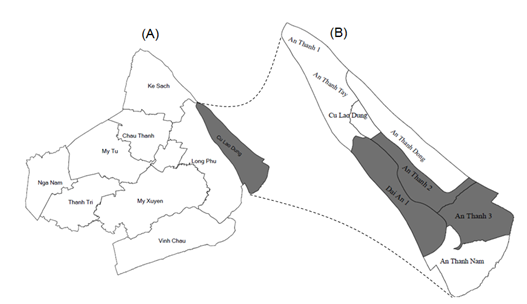
Figure 1 Location map of the study sites. (A) Indicates the map of Soc Trang province. (B) Indicates the map Cu Lao Dung district and the selected communes.

Status of farming system conversion from sugarcane to shrimp in Cu Lao Dung district

Due to being an islet of Hau River with a large part of the coastal area, Cu Lao Dung district has favorable conditions for marine and brackish water aquaculture. Shrimp farming has been established in Cu Lao Dung since the early 2000s, in particular in the coastal communes under the guideline and development plan of the district and province. However, the seawater intrusion has become increasingly serious, which has impact on the district’s agricultural production. Especially, the sugarcane area is severely affected. According to the report on the damage caused by salinity intrusion in An Thanh 3 commune, Cu Lao Dung district in 2015, the total area of agricultural production affected is 1,127 ha (damage level is 30% or more), of which sugarcane area is 1,124 ha, accounting for over 99.8%. In that context, during the past five years (since 2012), many farmers along the Hau River of the district have converted the farming system from sugarcane to shrimp. However, this changing has not generally brought about high efficiency because in the early time of transition, farmers face many risks in the production such as seed, technology and output market. According to People committee of Dai An 1 commune‘s report on socio-economic performance in 2015 and the direction and tasks in 2016, the total area of shrimp having profit is 49.3% (about 108.6 ha) while the proportion of areas with the breakeven and loss is 37.9% and 12.8%, respectively. Following field survey’s results, the experience of households in the study site in producing shrimp is only about 5 years. The major technical information source was from neighbors (98% of all respondents), only 17% of respondents indicated that they had access to new technical information from extension officers. Considering the production scale, on average, each household has about two ponds for shrimp farming with an area of about 0.55 ha. The mean of producing crop is two (2) crops / year, but there have farms with more intensive production, up to four crops / year. The economic performance of the changed farming system to shrimp in Cu Lao Dung district is shown in Table 1.

The results in Table 1 show that such indicators of shrimp converting farms as revenue, total cost, and profit vary among households due to large standard deviation and big gap between max and min values, suggesting that changed farming system is risky. Although the average profit is high, about 420 million/ha, the standard deviation (652 million) is much higher than the mean, pointing out that although many farmers are profitable, there are also many farmers suffering losses. The profit / total cost ratio was only 0.64, indicating that one VND of total cost invested can make only 0.64 VND of revenue. With high investment costs, if losses happen it will be very difficult for farmers to continue reinvesting. In order to help the policy makers and the farmers identify and mitigate risks in production, the study will continue to analyze the cost structure of the shrimp culture system at the study site.

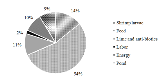
Figure 1 shows the structure of shrimp culture costs at the research area. The results reveal that feed cost accounted for the highest proportion (54%) of the total cost of shrimp culture in Cu Lao Dung district, followed by cost of breeding 14%, lime and antibiotics (11%), fuel cost (10%), pond depreciation expense (9%), and hired labor cost (2%). As such, if there have risks in the production, biggest losses are food and seed costs. Therefore, in order to limit the farmer's financial risk, it is necessary to identify good seed sources and optimal levels of feed. To better understand the risks faced by farmers in the production, the results in Figure 2 will show the level of risk from weather to production techniques and consumption.

Figure 2 The cost shares of shrimp farming.
Source: Authors’ calculation from household survey in 2016, n = 90.

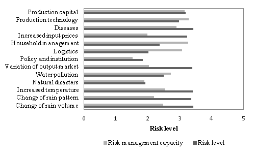
Figure 3 shows that shrimp farms in the study area encountered many risks in the production and the level of risk of each criterion is relatively high. The highest risk indicators are disease outbreaks, changes in rainfall and the rainy season calendar, high temperatures and fluctuations in the output market, the average for five criteria is about 3.4 (on a scale of 5). Criteria with a low level of risk in terms of people's perception of production are policies, institutions, logistics and natural disasters, which have an average score of about two. According to the results of the study, it was found that the households who had loss at least one time accounted for 91%. This data shows that the risk in shrimp farming is quite high. The main causes for losses are diseases, seed quality, weather changes and market fluctuations. Regarding the management capacity of farmers, the research results show that for the criteria of high risk, the farmers’ management ability to respond to the disease is quite good due to the support from professional staffs of agricultural extensions and companies. Some large-scale farms have hired fisheries specialists to manage the production, therefore technical issues are generally good. However, the capacity to manage issues related to weather and climate change, which is one of the criteria having large impact on shrimp culture, is rather limited. Thus, managers and scientists need to pay attention to this aspect in order to improve the adaptive capacity of shrimp farmers.

Figure 3 Types of risk and risk management of households.
Source: Authors’ calculation from household survey in 2016, n = 90.
Note: scale 1 to 5, where 1 is the lowest and 5 is the highest.

Technical and environmental efficiency

As mentioned above, this study applied stochastic frontier analysis to estimate technical and environmental efficiency of shrimp farms in the study site. Before calculating these efficiencies, it is essential to identify inputs and output of shrimp culture. The inputs and output of shrimp culture were described in Table 2.

Field survey’s results reveal that shrimp culture has three environmentally detrimental inputs including food (Z₁), medicine (Z₂) and fuel (Z₃) as well as two normal inputs such as seed (X₁) and labor (X₂). Environmentally detrimental inputs will cause environmental pollution if used excessively. For example, if farmers overuse food due to poor management techniques, this may lead to eutrophication due to the dense of organic components. Medicine abuse can negatively affect the living and development of other species in the water environment. Most of the fuels used are fossil fuels such as gasoline and oil, which, in the course of use, emits gases that pollute the environment as well as public health.

The output of shrimp culture in this research is shrimp yield per ha in a year. Other outputs in the production will not be considered in this study because they are very few. The main subject of the household is shrimp, so other outputs, such as fish and crabs, can be termed as the result of ecological blessedness, which does not reflect production technology of the households. Table 2 indicates that output and inputs of shrimp models in the research area have large variation. The reason is the influence of weather and difference in farms’ management level and seed source, the level of farms ‘success and failure is also different. This variation caused few estimates from SFA model using maximum likelihood estimation have statistical significance. Estimate results of production function were shown in Table 3.

Based on frontier production model’s estimation and using Equations (2) and (8), we can calculate output-oriented technical efficiency and environmental efficiency of shrimp farms. The distributions of these efficiencies were presented in Table 4 & Table 5.

Table 4 shows that the average output-oriented technical efficiency of shrimp farms in the study area was 72.74%, suggesting the farms could increase 27.26% of shrimp yield with current inputs used. Technical efficiency scores largely varied among households. The maximum efficiency level was 91.65% while the min was only 34.59%. These results indicate that many shrimp households face high risks in the production so the output-oriented technical efficiency is low. Most of shrimp farms achieve technical efficiency in the range from 70% to 90%, accounting about 66% of total sample observations. Households with efficiency level less than 70% occupied about 30% of total sample. The continuing part will discuss about environmental efficiency that was pointed out in Table 5.

The study found that on average, environmental efficiency of shrimp farms was 65.44%, indicating the farms have ability to reduce 35% of environmental detrimental inputs (food, medicine, fuel) without compromising current shrimp yield while holding other inputs constant. Similar with output-oriented technical efficiency, environmental efficiency of shrimp farms also has great variation, showing that the difference in production techniques of the shrimp households was quite large.

In general, the technical and environmental efficiency of the changed farming system is relatively low and variable. These results explicitly indicate that shrimp households in the study areas face high risks and inefficiency in resource use.

The research results also found that the average profit of changed farm system in the study sites was 419 million VND/ha. However, there has a large variation in profit among households, reflecting that the shrimp converting farms encounter risks in the production. The study also reveals that households who have suffered at least one time of loss account for 91% and the main causes of losses are diseases, seed quality, weather changes and market fluctuations. Moreover, indicators having the highest risk level are disease, changes of rainfall and rainy season calendar, high temperature and fluctuation of the output market, the average score of these criteria is about 3.4. However, the transformed shrimp farmers’ risk management capacity associated with weather and climate changes is still limited. Therefore, it is necessary to have suitable policies to improve the adaption ability for shrimp farmers in the research sites. The mean output-oriented technical efficiency of surveyed farms was 72.74%, pointing out that the farms have ability to increase shrimp yield by 27.76% with present inputs application. On average, environmental efficiency of the farms was 65.44%. This result suggests that bad inputs of shrimp culture having negative impacts on environment such as food, medicine, and fuel could be contracted about 35% without losing current level of shrimp yield in the condition of fixing other inputs. However, the research still has limitation, which did not identify determinants causing the difference in technical and environmental efficiency of transformed shrimp farms to recommend suitable policies. This limit will be the topic of the authors’ next study.

This study is funded in part by the Technical Cooperation Project "Building capacity for Can Tho University to be an excellent institution of education, scientific research and technology transfer" of JICA.

Authors declare there is no conflict of interest.

1. Carew–Reid J. Rapid assessment of the extent and impact of sea level rise in Viet Nam. Australia: International Centre for Environment Management (ICEM). 2008(82):1–82.
2. Wassmann R, Hien NX, Hoanh CT, et al. Sea level rise affecting the vietnamese mekong delta: Water elevation in the flood season and implications for rice production. Climatic Change. 2004;66(1–2):89–107.
3. Dasgupta S, Meisner C, WheelerD, et al. Pesticide poisoning of farm workers–implications of blood test results from vietnam. International Journal of Hygiene and Environmental Health. 2007;210:121–132.
4. Ecobichon DJ. Pesticide use in developing countries. Toxicology. 2001;160(1–3):27–33.
5. Reinhard S, Knox Lovell C, Thijssen GJ. Environmental efficiency with multiple environmentally detrimental variables; estimated with sfa and dea. European Journal of Operational Research. 2000;121(2):287–303.
6. Reinhard S, Lovell CK, Thijssen G. Econometric estimation of technical and environmental efficiency: An application to dutch dairy farms. American Journal of Agricultural Economics. 1999;81(1):44–60.
7. Reinhard S, Thijssen G. Nitrogen efficiency of dutch dairy farms: A shadow cost system approach. European Review of Agricultural Economics.2000;27(2):167–186.
8. Dung NH, Dung TTT. Economic and health consequences of pesticide use in paddy production in the mekong delta, vietnam. Economy and environment program for Southeast Asia (EEPSEA). 1999;1–39 p.
9. Aigner D, Lovell CA, Schmidt P. Formulation and estimation of stochastic frontier production function models. Journal of Econometrics. 1977;6(1):21–37.
10. Meeusen W, Broeck JV. Efficiency estimation from cobb–douglas production functions with composed error. International economic review. 1977;18(2): 435–444.
11. Tu VH, Yabe M, Trang NT, et al. Environmental efficiency of ecologically engineered rice production in the Mekong Delta of Vietnam. Journal of the Faculty of Agriculture, Kyushu University. 2015;60(2):493–500.
12. Tu VH. Estimating environmental efficiency for agricultural production: A case study of rice. Journal of Scientific Research and Development. 2015;13:1519–1526.
13. Tu VH. Resource use efficiency and economic losses: Implications for sustainable rice production in vietnam. Environment, Development and Sustainability. 2017;19(1):285–300
14. IAR1. Project: Control of aquatic environment pollution (shrimp and pangasius) by 2020. Vietnam: Institute for Aquaculture Research 1; 2013.
15. Tan LM. Impact assessment to the water quality at cangio shrimp–farming area. Vietnam: Science & Technology Development; 2006.
16. Farrell MJ. The measurement of productive efficiency. Journal of the Royal Statistical Society. Series A (General). 1957;120(3)253–290.
17. Jondrow J, Lovell CK, Materov IS, et al. On the estimation of technical inefficiency in the stochastic frontier production function model. Journal of econometrics.1982;19(2–3):233–238.
18. Coelli TJ, Rao DSP, O'Donnell CJ, at al. An introduction to efficiency and productivity analysis. Germany: Springer; 2005.
19. Kumbhakar SC, Lovell CK. Stochastic frontier analysis. UK: Cambridge University Press; 2003.
20. GSO. Statistical yearbook of Vietnam 2015. Vietnam: General Statistical Office; 2016.
21. STSO. Statistical yearbook of soc trang 2016. Vietnam: Soc Trang Statistical Office; 2016.