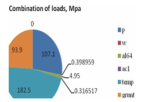
Designed loads on the sea buried pipeline include internal pressure of the product (natural gas), temperature of the transported product, and weight load of the medium. Certain operating conditions may lead to strength-threatening tension in the subsea pipeline, which is instantaneous us under static and dynamic random exposures. Load analysis of the main combination is shown in Figure 1 (note: sea buried pipeline is an object of the analysis). The purpose of this study is to evaluate damages of the natural gas pipelines due to fatigue caused by cyclic fluctuations of transportation temperature which contribute to defect growth.


Figure 1 Analysis of sea buried pipeline loads effect on specific combination; where p is a working pressure load, w is a dead weight load, temp–- is temperature impact, al64 is seismic load.
Mathematic model
There is a linear relationship between the input impacts combination and the output process
(1)
where С -may be constant or random values.
Mathematic model of the subsea pipeline vibrations under random operating and seismic loads can be described by a linear stochastic operator
(2)
After dividing the variables we have two independent differential equations. The first equation determines free vibrations of the system.1 The second is equation of pipeline vibrations in generalized coordinates under seismic load and operating parameters of the transported product;
(3)
Let us analyze the pipeline operating loads (internal pressure, temperature effect) as random processes. Here we should determine spectral density of all random processes from operating and seismic loads:
(4)
where
is response spectrum under seismic load,
is vibration spectrum of temperature effects. The
third summand in the equation (4) can be treated as an interference element, which makes additional contribution due to correlation. Let us write the equations of pipeline vibrations when exposed to a sum of loads a used by a random seismic load and variation of the parameters of the transported
(5)
By solving the equation (5), let us determine the roots of the standard equation:
(6a)
(6b)
Calculate transfer function of the equation
Let us calculate transfer function of the equation (5), assuming that
and solving the resultant equation:
Transfer function is described by the equation
(7)
Joint spectral density of random functions (t) and
can be calculated on the basis of the following assumption:
(8)
Considering the transfer function (7), the joint spectral density can be defined as
(9)
where <
is spectral density of temperature fluctuations of the product.
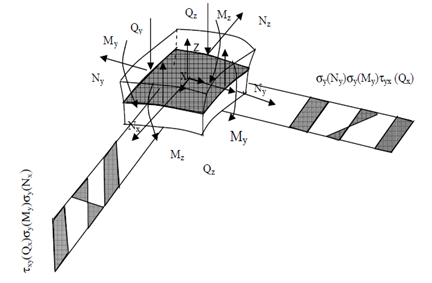
Stress-strain state of the pipeline shell can be evaluated using a finite element method. Internal stresses are associated with the loads on the pipeline wall shown in Figure 2.

Figure 2 Loads and stresses in the section of the pipeline shell: where N are longitudinal stresses in the pipeline wall, М,Q - bending moments and shearing stresses are distributed along the pipeline wall symmetric with respect to mid-surface of the shell.
Let us analyze random stationary external impact on the wall of the offshore pipeline. A relation linking tensor of the random strain with equivalent stress is called von Mises equation.2–4
(10)
We can evaluate probabilistic characteristics of there and nonequivalent stressed state in time and spectral ranges.
Matrix representation of stress on pipeline
Let us have matrix representation of an expression for
:
(11)
Then , where according to5
(12)
At tri axial compression or tension
Stressed state in a point
of the pipeline is a multidimensional random process with the six time-varying components. Equivalent stresses are considered to be strength criteria of the pipeline design as per von Mises criterion.4
The equivalent stress
in the point n of the pipeline under review determines fatigue life of the pipeline.
In practice, the pipelines operated in seismic areas are often exposed to random loads, insofar as the external impact parameters are stochastic here. The distributed static load leading to a dangerous stressed state in the pipeline wall is restricted by the maximum allowable load.
Let us describe a sea buried pipeline as a linear system. Seismic damage is other than local damage, as an increase in the pipe curvature is observed along the fixed sections.
This study focuses on designed pipeline risk assessment by virtue of the theory of runs.
Average number of runs
within level
is calculated by formula:
(13)
Failures may be treated as independent accidental events and estimated using a rare-event probability equation.
The conditional probability of the structural strain
exceeding the level a within the duration of an earthquake 0
t at least once is equal to:
(14)
The probability of the load F(t) to exceed the value Q0 within the duration Т at least once is equal to:
(15)
The required safety level of a structure
which supports the design seismic risk value Р* over the rated life Т0 is calculated by formula:
(16)
where
is the earthquake event frequency.
Reasonable structure reliability level is established on the basis of performance and reliability analysis carried out for existing structures; contingency analysis (for accidents occurred and simulated); and also on the basis of material resource efficiency considerations and safety requirements.
Cyclic variations of the transported product parameters can be recorded using linear addition hypothesis or Miner’s rule.5 This method has been developed to determine total damager ate П over a period of time Т caused by all loading cycles on the pipeline:
(17)
Where Nm is a number of intervals composing the measurement range
is a number of intervals composing the measurement range
,
is amplitude of stresses; Рki is repeat ability of full cycles that are in k range for
and j range for
; k=0.1,…,
c; j=0.1,…,
;
is a constant component of the cycle, where
is a minimum value
is a step for
is a step for
.
Flow chart of formula (17) implementation is shown in Fig.3.
Flow chart of total damage on pipeline
Flow chart of formula (17) implementation is shown in Figure 3.
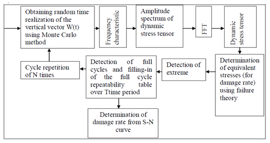
Figure 3 Flow chart of total damage rate determination of the pipeline design.
Pipelines having diameter to wall thickness ratio of higher than 20 mm are called thin walled, distribution of normal stresses that are perpendicular to the surface is uniform over the entire wall thickness. For isotropic materials stress-strain dependence is represented as follows under plane stress: follows:
(18)
For determination of internal stresses that appear in the walls of the offshore subsea pipeline under design loads a finite element model of the pipeline has been developed using solid finite elements. The internal stresses are calculated using finite element method and ANSYS software is present in Figure 1.
Pressure and temperature variation cycles associated with changes in natural gas transportation modes were simulated using a technique represented in Figure 3.
Calculations previously made for the non-buried pipeline as shown in demonstrated that the total damage rate Di for all wave loads was D=0.026,А=1.5741014, considering that service lifeТ=38.4years.6
At the stage of designing the subsea pipelines in the Caspian Sea, the decision was taken to bury the pipelines with consideration of seismic hazard. Based on the calculations it was decided to bury the subsea pipelines in the landfall sections to ensure protection from cycling waves.5 Nore searches of the fatigue parameters of the buried offshore subsea pipelines were made. We can determine total damage rate of the pipelines using technique from Figure 3. Combination of the subsea pipeline loads present on Figure 1 (shown as a percentage in the diagram).6–10
It is necessary to perform researches to determine pipeline fatigue. This article covers evaluation of the fatigue of the buried subsea pipelines. The fatigue calculations of the sea buried pipelines are made using simplified formulas to evaluate the fatigue rate of the underground pipelines. This method is not fully applicable to the operating mode of the buried offshore subsea pipelines (Figure 1). Simplified method of fatigue staring the valuation using Weibull distribution for simulation of the long-term fatigue stress distribution is described in the guidelines.2
Cumulative stress distribution function can be expressed as follows:8,9
(19)
Where Q is probability of stress range exceedance
; h are parameters of Weibull distribution; q is Weibull scale parameter, it is determined for the stress range,
:
(20)
Where
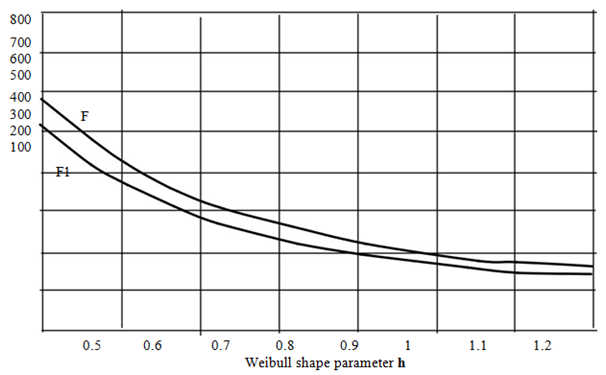
is stress range of n0 cycles. According to the technique,11 Weibull distribution parameters h are determined using linear interpolation of the stress range for values (0.90÷1.0) from the Table 1 for the curves S-N We can calculate duction factor of the allowable stresses from the curve F1, it’s present on Figure 4. Considering corrosion protection of the pipeline from the Table 2 we obtain14 a reducing factor of 0.19. In this case the stress reduction will be within
82.501 МPa for
=485.3.11–21
S-N |
Weibull shape parameter h |
|
|
|
|
|
curves |
0.50 |
0.60 |
0.07 |
0.80 |
0.90 |
1. 00 |
1.10 |
1.20 |
F1 |
523.3 |
376.7 |
289.9 |
233.9 |
196.4 |
169.6 |
149.6 |
134.3 |
Table 1 Allowable extreme stress range during 108 cycles for components in seawater with cathodic protection21

Figure 4 Allowable extreme stress range during 108 cycles for components in seawater with cathodic protection.21
Fatigue damage Utilization
|
|
Weibull shape parameter |
|
|
|
|
0.5 |
0.6 |
0.7 |
0.8 |
0.9 |
|
1 |
1.1 |
1.2 |
0.1 |
0.497 |
0.511 |
0.526 |
0.54 |
0.552 |
|
0.563 |
0.573 |
0.582 |
0.2 |
0.609 |
0.62 |
0.632 |
0.642 |
0.652 |
|
0.661 |
0.67 |
0.677 |
0.22 |
0.627 |
0.638 |
0.648 |
0.659 |
0.668 |
|
0.677 |
0.685 |
0.692 |
0.27 |
0.661 |
0.676 |
0.686 |
0.695 |
0.703 |
|
0.711 |
0.719 |
0.725 |
0.3 |
0.688 |
0.697 |
0.706 |
0.715 |
0.723 |
|
0.73 |
0.737 |
0.743 |
0.33 |
0.708 |
0.717 |
0.725 |
0.733 |
0.741 |
|
0.748 |
0.754 |
0.76 |
0.4 |
0.751 |
0.758 |
0.765 |
0.772 |
0.779 |
|
0.785 |
0.79 |
0.795 |
0.5 |
0.805 |
0.81 |
0.816 |
0.821 |
0.826 |
|
0.831 |
0.835 |
0.839 |
0.6 |
0.852 |
0.856 |
0.86 |
0.864 |
0.868 |
|
0.871 |
0.875 |
0.878 |
0.67 |
0.882 |
0.885 |
0.888 |
0.891 |
0.894 |
|
0.897 |
0.9 |
0.902 |
0.7 |
0.894 |
0.897 |
0.9 |
0.902 |
0.905 |
|
0.908 |
0.91 |
0.912 |
0.8 |
0.932 |
0.934 |
0.936 |
0.938 |
0.939 |
|
0.941 |
0.942 |
0.944 |
1.00 |
1.000 |
1.000 |
1.000 |
1.000 |
1.000 |
|
1.000 |
1.000 |
1.000 |
Table 2 Reduction factor on stress to correspond with utilisation factor
for C - W3 curves14
Let us analyze the sea buried pipeline laid on the bottom of the Caspian Sea. The pipeline is buried and its designed service life is 30 years. Taking into account the allowable stresses14
=485.3 MPa, stress reduction will be as follows:
Fatigue damages reduce the allowable stresses by 17%.Additional distinguishing marks to be added to the character of classification of steel subsea pipelines present in Table 3.14
Pipeline class |
|
L , LI |
1,5 |
L2 |
1,65 |
L3 |
1,8 |
G , Gl |
1,4 |
G2 |
1,5 |
G3 |
1,65 |
Table 3 Strength factor
for pipeline pure buckling calculation
The stress value of 402.799 MPa is obtained from the Table 4 of the standards14 using ne(G3) coefficient of 1.33 and considering k coefficient of 0.864 from the Table 4. For the pipeline having diameter of 406.4mm and wall thickness of 14.5 mm the allowable stress range is 261.66 MPa.22–26
Pipeline |
|
|
class |
For normal operational conditions |
For short - term loads during construction and hydraulic tests |
L , LI |
0,8 |
0,95 |
L2 |
0,727 |
0,864 |
L3 |
0,696 |
0,826 |
G , Gl |
0,8 |
0,95 |
G2 |
0,762 |
0,905 |
G3 |
0,727 |
0,864 |
Table 4 Strength factors in terms of total stresses
The allowable stress for the pipeline is 255.6 MPa.14 The result obtained does not exceed the allowable level but we still have 2.3% to reach the allowable stress level. Requirements of standards4,9 are used in the calculation. To evaluate fatigue of the buried subsea pipeline, it is required to carry out fatigue tests of the pipelines in order not to rely on standard coefficients in the calculations when evaluating strength of the pipelines during the design stage and not to contemplate about probable margin of the allowable stresses.


