This paper explores patterns and stability of the air-water thermal gravitational convection in a thin and wide horizontal container whose top and bottom walls are adiabatic while vertical sidewalls have prescribed different temperatures. A compact polynomial solution describes a slow multi-cell motion and a temperature distribution away from the sidewalls. The solution explicitly shows how the flow topology depends on the water fraction, thermal surface-tension effect, characterized by the Marangoni number Ma, and buoyancy strength characterized by the Grashof number Gr. The performed numerical simulations agree with the analytical solution for small Gr and Ma and describe changes in the flow topology for large Gr and Ma. The flow transforms into a boundary-layer pattern with jets located near the interface and container walls. The jet entrainment generates new cells in the bulk water flow. As Ma increases, the Marangoni stresses focus near the sidewalls and develop a thin thermal boundary layer near the cold wall. The performed stability study reveals that the steady convection is stable for Gr and Ma values considered. The stability is due to the favorable stratification of water density provided by the adiabatic walls. The results can be utilized for the development of efficient heat exchangers.

Keywords: Thermal Gravitational Convection; Two-Fluid Flows; Side Heating; Marangoni Number; Grashof Number; Prandtl Number; Marangoni Stresses; Czochralski Technique; Surface-Tension; Boussinesq Approximation; Boundary Conditions; Adiabatic Condition; Jacobians.

Gr: Grashof Number; Ma: Marangoni Number; Pr: Prandtl Number

Convection in a horizontal layer of a fluid induced by the horizontal gradient of temperature is one of basic problems of heat transfer. The global circulation between the equatorial and polar oceanic regions occurs mostly due to the horizontal gradient of temperature.¹ Technological applications include shallow water pools used for the removal of waste heat, the Czochralski technique of crystal growth² and cooling systems for nuclear reactors and solar energy collectors.³

The problem also is of fundamental interest being a rare case where experimental, analytical, and numerical results allow meaningful comparison in a wide range of the flow strength, characterized by the Grashof number Gr (Table 1-3). This helped understand the flow physics and explain the generation of cells by the jet entrainment mechanism in the single-fluid convection.⁵ Our paper shows that the jet entrainment mechanism works in the two-fluid convection as well. It is striking that these flows are stable for large Gr despite the presence of inflection points in the velocity distribution.

For small and moderate Gr, a single-fluid flow in a rectangular container away from its vertical walls excellently agrees with the elegant polynomial solution obtained by Ostroumov:⁶

$u/u_{max}=(y^3-y){\left(27\right)}^{1/2}/2$ ,

where u is the horizontal velocity and u_max is its maximal magnitude; y is the vertical coordinate, divided by the layer half-height. The horizontal walls are located at $y=\pm 1$ . Birikh⁷ generalized this solution for the case where the upper surface is free and subject to the thermal surface-tension (Marangoni) effect. Multi-fluid convection is systematically analyzed in the monograph by Nepomnyashchy et al.⁸ Chapter 5 of book⁸ describes multi-layer analytical solutions for prescribed temperatures of horizontal boundaries. In contrast, our paper addresses the adiabatic horizontal walls. The stability features are very different in these two cases.

 We show that the flow stability radically depends on boundary conditions at the horizontal walls. If temperature is prescribed at the walls, the flow becomes unstable for rather small Gr. Birikh⁹ considered the stability of flow⁶ at the Prandtl number $Pr=0$ and found that the critical value of the Grashof number is Gr* = 495. Gershuni et al.¹⁰ explored the stability of flow⁶ at Pr > 0 with respect to two-dimensional¹⁰ and three-dimensional¹¹ disturbances.

They predicted two kinds of instability:

1. Shear-layer K-instability related to the existence of inflection point in the u(y) profile and
2. Thermal R-instability caused by the unstable density stratification near the horizontal walls; here K is for Kelvin and R is for Rayleigh. As Pr increases, the K-instability disappears for Pr > 0.5, but the R-instability occurs for any large Pr.

In contrast to these predictions, the experimental studies^2,4 reveal no instability up to $Gr\approx 4\times {10}^7$ . As Gr increases, the flow transforms from that described by solution⁶ to the boundary-layer pattern with jets developing near the container walls and a slow multi-cellular motion in the bulk region surrounded by the jets.

It is paradoxical that no instability occurs despite the u(y) profile becomes wavy with a few inflection points.^2,4 This paradox was recently explained.¹² The horizontal walls have prescribed temperatures in the stability studies^8-10 while the walls are nearly adiabatic (no heat flux) in the experiments.^2,4 It is revealed that the R-instability disappears if the boundary conditions change from the fixed-temperature to the adiabatic ones.¹² The physical reason is that the density stratification becomes stable in the entire flow domain for the adiabatic conditions. This clarifies why no instability is observed in the experiments.^2,4

The analytical solution⁶ was generalized for the cylindrical geometry and the centrifugal force replacing the gravity. For a small axial gradient of temperature, the centrifugal convection in a rotating pipe is also described by the polynomial solution:¹³

$w/w_0=1-4r^2+3r^{4}and(T-T_1)/(T_0-T_1)={(1-r^2)}^3$ ;

where r is the distance from the axis divided by the pipe radius. Subscripts 0 and 1 denote values of axial velocity w and temperature T at the axis and sidewall respectively. There is also analytical (though not polynomial) solution for a gap between two co-rotating pipes.¹³ For a narrow gap, the cylindrical problem becomes close to that for a horizontal layer.⁶ Birikh and Pukhnachev¹⁴ generalized the solution¹³ to describe a two-fluid thermal convection with the Marangoni effect taken into account. The numerical simulations of the air-water centrifugal convection in a cylindrical container¹⁵ agree with the analytical solutions and help explain the emergence of new flow cells due to the Marangoni effect. A similar development occurs in the two-fluid flow studied here.

Early theoretical and experimental studies of thermal convection in a two-fluid horizontal layer are mostly related to vertical heating.^8,16 To our knowledge, the first experimental study for lateral heating was performed by Sparrow et al.¹⁷ for the water-hexanol horizontal layer. Villers & Platten¹⁸ measured the velocity profiles in each fluid layer as a function of the height in a system formed by water and heptanol and analyzed the solutions for an elongated layer¹⁹ The polynomial solutions^6,7 easily can be generalized for a multi-fluid convection in a horizontal layer.⁸ Doi & Koster²⁰ studied theoretically the thermo-capillary convection under microgravity conditions in two immiscible liquid layers with a free upper surface. In addition, they carried out numerical simulations in a box of aspect ratio 4 in order to analyze the effect of the vertical walls. Numerical simulations in cavities of different aspect ratios for coupled thermos-capillary and buoyancy-driven convection were performed by Liu et al.,²¹ and an asymptotic solution for the velocity in the limit of infinite aspect ratio and zero gravity has been derived ²²

Madruga et al.¹⁶ investigated flow patterns in an unbounded horizontal layer of two liquids and studied the flow stability. Our work generalizes their study by also addressing a bounded layer and differs from^8,16 by the following features:

1. The horizontal walls are adiabatic here while they have prescribed temperatures.^8,16 This difference is crucial for the flow stability as discussed above.
2. We focus on the air-water flow motivated by applications for cooling systems³ while the fluids are specific for crystal-growth applications in¹⁶and the other above cited works.
3. A compact form of the base-flow solution is derived. This form explicitly shows whether the flow patterns are single-cellular or two-cellular in both fluids.
4. A pattern map on the parametric plane (the Marangoni number, the relative height of the interface) is obtained with analytically determined boundaries between regions of different flow topologies.
5. Our study also considers the two-dimensional (2D) flow in a container of aspect ratio 4 and describes the development of jet-like boundary layers near the container walls and the interface. We argue that eddies emerging in the bulk flow are generated by the jet entrainment.
6. The stability of the one- and two-dimensional flows is explored.
7. In the rest of this paper, we formulate the problem in Section 5, describe the polynomial solutions in Section 6, the numerical technique in Section 7, explore the slow 2D flow in Section 8, effects of increasing Gr (Section 9) and Ma (Section 10), investigate the stability of the core (Section 11) and two-dimensional (Section 12) flows, and summarize the results in Section 13.

Flow geometry

Consider a rectangular container of length l and height h schematically shown in Figure 1. The origin of horizontal (x) and vertical (y) axes is located at the left lower container corner and the z-axis is normal to the picture plane in Figure 1. Velocity and temperature of the base flow is time and z-independent. Using h as a length scale makes the coordinates dimensionless.

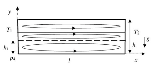
Figure 1 Schematic of the problem.

The container is filled with a heavy fluid (here water) occupying the region, $0<y<H_i=h_i/h$ , and with a light fluid (here air) occupying the region, $H_i<y<1$ ; g is the gravity acceleration; $y=H_i$  is the interface, depicted by the bold dashed line in Figure 1. The interface deformation is neglected here based on the experimental observation²that the deformation is very small. The left (right) wall has prescribed temperature$T_1\left(T_2\right);T_1<T_2$ . The top and bottom walls are adiabatic. The temperature difference and gravity circulates both fluids. The arrowed contours in Figure 1 depict a possible flow pattern which depends on the fluid properties and fractions.

It is convenient to introduce the dimensionless temperature,

$\vartheta =({\rm T}-{{\rm T}}_m)/(\epsilon {{\rm T}}_m),{{\rm T}}_m=\left({{\rm T}}_1+{{\rm T}}_2\right)/2,\epsilon =({{\rm T}}_2-{{\rm T}}_1)/{{\rm T}}_m$ (1)

With no flow, the temperature distribution is

$\vartheta ={\vartheta }_0=-1/2+x/L, 0\le x\le L,$                            (2)

where L = l/h is an aspect ratio of the container.

• Boussinesq approximation

We apply the Boussinesq approximation,

$\rho /{\rho }_m=1-\epsilon \beta \vartheta ,$                (3)

$\beta =-{\rho }_m{}^{-1}{T}_m\partial \rho /\partial T,$          (4)

The quantities, characterizing the heavy (light) fluid, are marked hereafter by subscript “h” (“l”). Equations and relations, which serve for both fluids, are unmarked. In relations (3) and (4), $\rho$ is a density, ${\rho }_m$  is its value at $T={{\rm T}}_m=\left({{\rm T}}_1+{{\rm T}}_2\right)/2$  and $\beta$  is a dimensionless thermal expansion coefficient. For the Boussinesq approximation to be valid, density variations must be small compared with ${\rho }_m$  i.e., $\epsilon \beta <<1$ . To this end, we take T_m = 300K = 27°C, T₁ = 18°C and T₂ = 36°C. This yields that$(T_2-T_m)/T_m=0.03$ , $(T_1-T_m)/T_m=-0.03$  and$\epsilon =0.06$ . For example, ${\beta }_h=0.082$ at T_m = 300K and $\epsilon {\beta }_h=0.00492$  for water and ${\beta }_1=1$ and $\epsilon {\beta }_1=0.06$  for air. Therefore, the Boussinesq approximation is applicable. The Grashof number is$Gr=\epsilon \beta g{h}^3/{\nu }^2$ , the Prandtl number is $Pr=\nu /\kappa$ and the Rayleigh number is Ra = GrPr; $\nu$  is a kinematic viscosity and $\kappa$  is a thermal diffusivity of a fluid. We address here a water-air flow. At the atmospheric pressure and T = T_m, the fluid properties are listed in Table 4.

Governing equations

 Using$h,h^2/\nu ,\nu /h,{\rho }_m{\nu }^2/h^2$ , as scales for length, time, velocity, and pressure, respectively, renders all variables dimensionless. Then the Boussinesq equations have the form:

$\partial u/\partial x+\partial v/\partial y+\partial w/\partial z=0,$          (6)

$\partial u/\partial t+u\partial u/\partial x+v\partial u/\partial y+w\partial u/\partial z= -\partial p/\partial x+{\partial }^{2}u/\partial x^2+{\partial }^{2}u/\partial y^2+{\partial }^{2}u/\partial z^2,$ (7)

$\partial v/\partial t+u\partial v/\partial x+v\partial v/\partial y+w\partial v/\partial z=Gr\vartheta -\partial p/\partial y+{\partial }^{2}v/\partial x^2+{\partial }^{2}v/\partial y^2+{\partial }^{2}v/\partial z^2$                (8)

$\partial w/\partial t+u\partial w/\partial x+v\partial w/\partial y+w\partial w/\partial z= -\partial p/\partial z+{\partial }^{2}w/\partial x^2+{\partial }^{2}w/\partial y^2+{\partial }^{2}v/\partial z^2$                   (9)

$\partial \vartheta /\partial t+u\partial \vartheta /\partial x+v\partial \vartheta /\partial y+w\partial \vartheta /\partial z=[{\partial }^2\vartheta /\partial x^2+{\partial }^2\vartheta /\partial y^2+{\partial }^2\vartheta /\partial z^2]/Pr$        (10)

Where $(u,\nu ,w)$  are the velocity components in Cartesian coordinates (x, y, z), t is time, and p is pressure reduced by its hydrostatic contribution. The term $Gr\vartheta$ in (8) represents the buoyancy force. Equations (6)-(10) are applied for both light and heavy fluids using values of Gr and Pr corresponding to each fluid.

We denote the list $(u,\nu ,w,p,\vartheta )$ as V, and look for a solution of the system (6)-(10) in the form

$V=V_b\left(y\right)+a{V}_d\left(y\right)exp(i\alpha x+ikz-i\omega t)+c.c.,$             (11)

for a horizontal base flow away from the vertical walls as L ® ¥ and in the form

$V=V_b\left(x,y\right)+a{V}_d\left(x,y\right)exp(ikz-i\omega t)+c.c.,$                 (12)

for a two-dimensional base flow for finite L.

Subscripts “b” and “d” denote the base flow and a disturbance, respectively; c.c. denotes the complex conjugate of the preceding term; $a<<1$  is amplitude; real $\alpha andk$  are wave numbers; and $\omega ={\omega }_r+i{\omega }_i$  is a complex number to be found, ${\omega }_r$  is a frequency and ${\omega }_i$  is a growth rate of a disturbance. For a decaying (growing) disturbance, ${\omega }_i$  is negative (positive). For neutral disturbances$\omega =0$  . The equations governing the base flows result from substituting (11) or (12) in system (6)-(10) and setting a = 0. The terms of order O(a) constitute equations governing infinitesimal disturbances.

Boundary conditions

Equations (6)-(10) are solved under the following boundary conditions:

1. No-slip at all walls: u = v = w = 0 at y = 0, y = 1, x = 0 and x = L.
2. Fixed temperatures of vertical walls: ${\vartheta }_b=-1/2,{\vartheta }_d=0atx=0and{\vartheta }_b=1/2,{\vartheta }_d=0atx=L.$
3. Adiabatic conditions at the horizontal walls: $\partial \vartheta /\partial y=0aty=0andy=1.$
4. Continuity of temperature and velocity at the interface: ${\vartheta }_l={\vartheta }_h,u_h={\nu }_r{u}_l,v=0$  and $w_h={\nu }_r{w}_{l } at y=H_i;{\nu }_r={\nu }_l/{\nu }_h$  is the light-to-heavy fluid kinematic viscosity ratio.
5. Continuity of heat flux at the interface: $\partial {\vartheta }_h/\partial y={\lambda }_r\partial {\vartheta }_l/\partial y$ , where ${\lambda }_r={\lambda }_l/{\lambda }_h$  is the light-to-heavy thermal conductivity ratio.
6. Continuity of tangent stresses at the interface: $\partial u_h/\partial y={\rho }_r{\nu }_r{}^2\partial u_l/\partial y-\epsilon M{a}_1\partial \vartheta /\partial xaty=H_i$ , where the left-hand-side term is the shear stress of heavy fluid, the first right-hand-side term is the shear stress of light fluid and the last term is the Marangoni stress; ${\rho }_r={\rho }_l/{\rho }_h$  is the light-to-heavy fluid density ratio; and $M{a}_1=-T_m\left(d\sigma /dT\right)h/({\rho }_h{\vartheta }_h{}^2)$  is the dimensionless value of $d\sigma /dT$  which is independent of $\epsilon andL$ . We use the Marangoni number in the form of$Ma=M{a}_1\epsilon /L$ . Condition (iii)-(vi) are applied for both base flow and disturbances.

The interface, y = H_i, is considered undisturbed here because this limitation simplifies the analysis and seems a reasonable approximation since no significant deformation of the interface was observed in the experiment.² Since equations (11)-(13) and boundary conditions for disturbances are uniform, there is the zero solution. For a non-zero solution, eigenvalues of w must be found.

Reduction of governing equations

The base flow is nearly x-independent near x = L/2 if L >> 1. Here, we consider the corresponding limiting case as L ® ¥ where velocity of both fluids is x-directed and depends on y only. In this one-dimensional problem, equations (6)-(10) reduce to

$\partial p/\partial x={\partial }^{2}u/\partial y^2,$               (13)

$\partial p/\partial y=Gr\vartheta ,$      (14)

$Pr.u\partial \vartheta /\partial x={\partial }^2\vartheta /\partial y^2$ .       (15)

Differentiating (14) with respect to x yields${\partial }^{2}p/\partial x\partial y=Gr\partial \vartheta /\partial x$ . Differentiating (13) with respect to y and substituting ${\partial }^{2}p/\partial x\partial y=Gr\partial \vartheta /\partial x$  gives

${\partial }^{3}u/\partial y^3=Gr\partial \vartheta /\partial x$ .         (16)

There is a solution for temperature in the form,

$\vartheta ={\vartheta }_0\left(x\right)+{\vartheta }_1\left(y\right)$ ,             (17)

where${\vartheta }_0$  is given by (2) and ${\vartheta }_1$  must be found. Therefore, $\partial \vartheta /\partial x=d{\vartheta }_0/dx=1/L$ . Substituting this in (16) yields

$d^{3}u/d{y}^3=Gr/L$ .               (18)

It is convenient to introduce stream function$Q\left(y\right),u=dQ/dy$ , which satisfies the equation,

$d^{4}Q/d{y}^4=24A, A=Gr/\left(24L\right)$ .   (19)

Parameter $A=(\epsilon /L)\beta g{h}^3/(24{\nu }^2)$  has the multiplier,$\epsilon /L$ , which is a dimensionless horizontal temperature gradient—a characteristic common for both fluids.

The boundary conditions are the no-slip at the walls, y = 0 and y = 1, and zero flow rate for each fluid:

$Q_h=d{Q}_h/dy=0aty=0and{Q}_h=0aty=H_i$ .      (20)

$Q_l=d{Q}_l/dy=0aty=1and Q_l=0aty=H_i$ .         (21)

The velocity continuity at the interface yields

$u_h={\nu }_r{u}_l aty=H_i$ .                             (22)

The shear stress continuity at the interface (condition vi), (17) and (2) yields

$d{u}_h/dy ={\rho }_r{\nu }_r{}^{2}d{u}_l/dy-Ma, {\rho }_r={\rho }_l/{\rho }_h$ .      (23)

Polynomial solution

Integrating (19) four times and satisfying conditions (20) yield that

$Q_h=A_h{y}^2(y-H_i)(y-y_h)$ ,               (24a)

where y_h is a constant to be found. The line y = y_h, where Q_h = 0, separates flow cells. Therefore, the heavy-fluid flow is two-cellular if 0 < y_h < H_i and one-cellular otherwise. Differentiating (24a) yields

$u_h\left(y\right)=A_h[4y^3-3y^2\left(H_i+y_h\right)+2y{H}_i{y}_h]$                  (24b)

and              $d{u}_h/dy=A_h[12y^2-6y\left(H_i+y_h\right)+2H_i{y}_h]$    (24c)

Therefore,            $u_h\left(H_i\right)=A_h{H}_i{}^2(H_i-y_h)$                  (24d)

And         $d{u}_h/dy\left(H_i\right)=A_h{H}_i(6H_i-4y_h)$                   (24e)

 Integrating (19) four times and satisfying (21) yield

$Q_l=A_l{(1-y)}^2(y-H_i)(y-y_l)$ ,                         (25a)

where y_l is a constant to be found. The light-fluid flow is two-cellular if H_i < y_l < 1 (as in Figure 1) and one-cellular otherwise. Differentiating (25a) gives

$u_l\left(y\right)=A_l(1-y)[(1-y)(2y-H_i-y_l)-2(y-H_i)(y-y_l)]$          (25b)

and differentiating (25b) gives

$d{u}_l/dy=2A_l[6y^2-3y\left(2+H_i+y_l\right)+1+2H_i+2y_l+H_i{y}_l].$      (25c)

This yields that   $u_l\left(H_i\right)=A_l{(1-H_i)}^2(H_i-y_l)$         (25d)

and $d{u}_l/dy\left(H_i\right)=2A_l(3H_i{}^2-2H_i{y}_l-4H_i+2y_l+1)=2A_l(1-H_i)(1-3H_i+2y_l)$    (25e)

 Constants y_h and y_l follow from conditions (22) and (23). Condition (22) results in       

$y_h=H_i-{\nu }_r{(1/H_i-1)}^2(H_i-y_l)A_l/A_h$           (26)

Finally, it follows from condition (23) that

$y_l=[H_i{}^2{A}_h/A_l+2{\nu }_r{(1-H_i)}^2+{\rho }_r{\nu }_r{}^2(1-H_i)(3H_i-1)+Ma/\left(2A_l\right)]/[2{\nu }_r(1-H_i)({\rho }_r{\nu }_r+1/H_i-1)]$ . (27)

 The relations (24a), (25a), (26) and (27) explicitly describe the stream function and velocity profiles as well as the number and arrangement of flow cells.

One and two-cell light-fluid flows

Since A_h, A_l and Ma have the multiplier, $\epsilon /L$ , the flow strength in both fluids is proportional to $\epsilon /L$  while y_h and y_l are $\epsilon /L$  -independent. For H_i close to 1, the motion of both fluids is one-cellular. The heavy-fluid circulation is driven by the thermal buoyancy force and by the Marangoni stresses. The light-fluid circulation is driven by the heavy-fluid motion. The thermal-buoyancy effect is negligible for the upper fluid.

However as H_i decreases, the buoyancy contribution rises in the light fluid and one more flow cell emerges near the top wall at Ma = Ma_l. The Ma_l value follows from (27) at y_l = 1:

$M{a}_l=2A_l[3{\rho }_r{\nu }_r{}^2{(1-H_i)}^2+2{\nu }_r{(1-H_i)}^3/H_i-H_i{}^2{A}_h/A_l]$ .     (28)

The light-fluid motion is singe- (two-) cellular for Ma > Ma_l (Ma < Ma_l).

Figure 2 depicts profiles of velocity u and flow rate Q in water (curves) and air (dots) at H_i = 0.5, A_h = 1, and at two values of the Marangoni number. At Ma = 0 (bold curves), the air flow is two-cellular. The motion in the lower air cell, H_i < y < y_l = 0.807, is driven by the water flow while the motion in the upper air cell, y_l < y < 1, is driven by air buoyancy as Figure 1 schematically depicts. With increasing Ma, the upper air cell shrinks to the top wall and disappears at Ma = Ma_l = 0.166 as the thin curves illustrate in Figure 2.

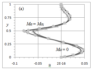
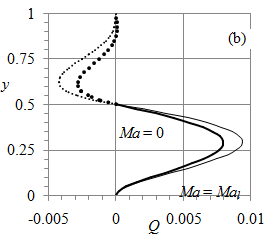
Figure 2 Dependence of (a) velocity u and (b) stream function Q on the vertical coordinate y at H_i = 0.5 and A_h = 1. The solid (dotted) curves correspond to the water (air) flow. Values of u and Q in air are multiplied by ν_r for convenient observation.The bold (thin) curves depict the results for Ma = 0 (Ma =0.166). Square and cross symb ols show numerical results at L = 4 and x = L/2.

Comparison of the thin and bold curves in Figure 2 shows that the Marangoni effect intensifies the water motion since the buoyancy and Marangoni effects cooperate in the water flow. The increased velocity magnitude at the interface speeds up the adjacent air flow expands the lower air cell and diminishes the upper air cell. For Ma ³ Ma_l, the entire air-water motion is driven by water buoyancy and the Marangoni effect while the effect of air buoyancy diminishes that results in the one-cellular air flow. The agreement between the analytical and two-dimensional numerical results verifies both of them. The numerical results (square and cross symbols in Figure 2) are discussed in more detail in Section 8.1.

Temperature distribution

Substitution of (17) and (2) in (10) yields$d^2{\vartheta }_1/d{y}^2=uPr/L$ , Taking into account that u = dQ/dy and integrating, we obtain that

$d{\vartheta }_1/dy=QPr/L$ ,                              (29)

with the adiabatic condition at the horizontal walls and the continuity condition for the heat flux at the interface being satisfied. According to equation (29), the heat flux is zero at the interface, i.e., no heat transfer occurs between the heavy and light fluids for the adiabatic walls.

Integrating (29) from y = H_i with the initial condition, ${\vartheta }_1\left(H_i\right)={\vartheta }_i$  yields the vertical distribution of temperature in both fluids:

${\vartheta }_h={\vartheta }_i+P{r}_h\left(A_h/L\right)[(y^5-H_i{}^5)/5-(y^4-H_i{}^4)\left(H_i+y_h\right)/4+(y^3-H_i{}^3)H_i{y}_h/3]$                 (30)

${\vartheta }_l={\vartheta }_i+P{r}_l\left(A_l/L\right)[(y^5-H_i{}^5)/5-(y^4-H_i{}^4)\left(2+H_i+y_l\right)/4+(y^3-H_i{}^3)\left(1+2H_i+2y_l+H_i{y}_l\right)/3-(y^2-H_i{}^2)\left(H_i+y_l+2H_i{y}_l\right)/2+(y-H_i)H_i{y}_l]$  (31)

Figure 3 depicts the temperature profiles, (30) and (31), for the flows shown in Figure 2. In contrast to the problem studied by Madruga et al.,¹⁶ where the temperature stratification is unstable near the bottom, here the stratification is stable: the colder (warmer) water is located near the bottom (interface). This feature should make the flow stable even for large Gr.¹²

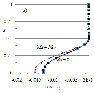
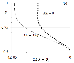
Figure 3 (a) Dependence of temperature, $\vartheta -{\vartheta }_i$ , on the vertical coordinate y at H_i = 0.5. The solid (dotted) curves correspond to the water (air) flow. The bold (thin) curves corresponds to Ma = 0 (Ma =0.166). Square and cross symbols show numerical results at L = 4 and x = L/2. (b) Close-up of (a) in the air flow.

The lower air cell at Ma = 0 and the entire air domain for $Ma\ge M{a}_l$  have unstable density stratification (Figure. 3(b)), but the temperature variation in the air region is negligibly small compared with that in the water region at H_i = 0.5. The agreement between the analytical and numerical (square and cross symbols in Figure 3) results verifies both our analytical and numerical calculations of temperature distributions.

Map of flow patterns

Figure 4 is a map of flow patterns. Curve 1 in Figure 4(a) depicts relation (28). Above curve 1, water and air flows are one-cellular as the upper inset in Figure 4(a) schematically shows. The air circulation is driven by the water circulation. Below curve 1 in Figure 4(a), the air flow is two-cellular as the lower inset in Figure 4(a) schematically shows where the bold dashed line denotes the interface. The new cell emerges near the top wall at Ma = Ma_l. The motion in the lower air cell is driven by the water circulation while the motion in the new cell is driven by the air buoyancy.

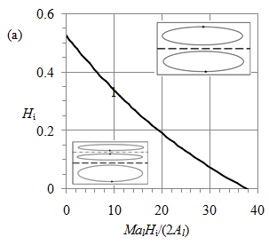
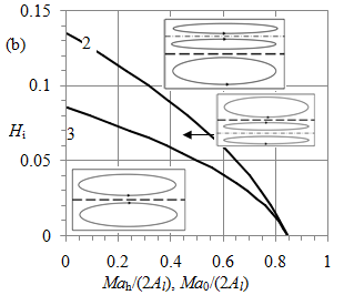
Figure 4 Dependence of air-water convection pattern (insets) on water fraction H_i and Marangoni number Ma. Curves 1, 2 and 3 depict relations (28), (32) and (33) respectively.

As H_i decreases at a fixed Ma, the air flow cell, driven by the water motion, shrinks, i.e., y_l decreases. At y_l = H_i, this cell collapses and the velocity at the interface becomes zero according to (25b), i.e., the interface affects the flow as a wall. It follows from y_l = H_i and (16) that y_h = H_i. Both air and water motions become one-cellular, each being driven by its buoyancy. Substituting y_l = H_i in (27) yields the corresponding value of Ma = Ma_h:

$M{a}_h= 2A_l{\rho }_r{\nu }_r{}^2{(1-H_i)}^2-2A_h{H}_i{}^2$ (32)

Curve 2 in Figure 4(b) depicts relation (32). Above curve 2, the flow topology is the same as below curve 1 in Figure 4(a). Below curve 2, i.e., for Ma < Ma_h, the water flow becomes two-cellular as the middle inset schematically shows in Figure 4(b) where the bold dashed line denotes the interface. Relation (26) yields that if y_l < H_i than y_h < H_i as well. This physically means that the air flow reverses the water motion near the interface developing the new water cell, y_h < y < H_i.

As H_i further decreases at a fixed Ma, the water cell, driven by the air motion, expands, i.e., y_h decreases down to zero. Substituting y_h = 0 in (26) and excluding y_l from (26) and (27) yield the corresponding value of Ma = Ma₀:

$M{a}_0=M{a}_h+4A_h{H}_i{}^2[1+{\rho }_r{\nu }_r{H}_i/(1-H_i)]$                     (33)

Curve 3 in Figure 4(b) depicts relation (33). For Ma < Ma₀, the water and air flows are one-cellular as the lower inset schematically shows in Figure 4(b). The water motion is driven by the air buoyancy. The water and air circulations in the region below curve 3 in Figure 4(b) are reversed compared with those in the region above curve 1 in Figure 4(a): the streamline topologies are identical, but the flow directions are opposite.

Stable stratification

At parameter values, corresponding to curve 2 in Figure 4(b), both air and water circulations are anticlockwise that makes the density stratification stable in both media. Since the water layer is thin compared with the air layer, H_i < 0.14, as Figure 4(b) illustrates, the temperature variation in the water is small compared with that in the air.

Figure 5 illustrates this feature depicting the vertical profiles of velocity and temperature, normalized by their maximal values, at H_i = 0.1 and Ma = 0.63A_l. This Ma value follows from relation (32). Since the velocity and temperature profiles are hardly visible in the water layer, 0 < y < 0.1, in Figure 5(a), they are scaled up in Figure 5(b). Figure 5 illustrates the stable density stratification in both air and water domains (dashed curves).

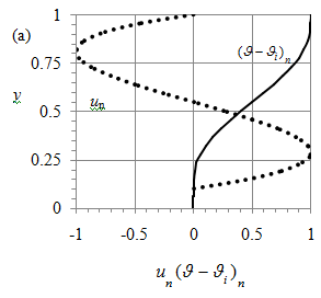
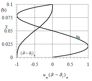
Figure 5 Profiles of normalized velocity u and temperature$\vartheta$  at H_i = 0.1 and Ma = Ma_h= 0.63A_l in (a) air and (b) water.

To simulate the nonlinear problem for (a) two-dimensional (2D) basic flows and (b) the generalized eigenvalue problem for the three-dimensional time-dependent infinitesimal disturbances, we use a numerical technique which is a variation of that described in detail in.²³ First, each variable (velocities, pressure and temperature) and all its spatial and temporal derivatives, which appear in equations (6)-(10) and the boundary conditions, are composed as a single symbolic vector.

For example, for the x-velocity in the water flow we create a vector having 8 components:

$x_w=[u_w,\partial u_w/\partial x,\partial u_w/\partial y,\partial u_w/\partial z,{\partial }^2{u}_w/\partial x^2,{\partial }^2{u}_w/\partial y^2,{\partial }^2{u}_w/\partial z^2, \partial u_w/\partial t]$ .

The next step is to use a symbolic toolbox to calculate the analytical Jacobians of all the equations with respect to all the symbolic vectors. Using these analytical Jacobians we generate functions which then are evaluated point by point in the air and water domains. In this procedure, we use the MATLAB procedure matlab Function to convert the symbolic Jacobians in MATLAB functions.

Then, we carry out the spatial and temporal discretization of the problem. For the 2D problem, the water and air domains are discretized using a set of n_h and n_l Chebyshev spectral collocation points in the vertical direction (along the y-axis in Figure 1). The water and air domains are discretized using a set of nx Chebyshev spectral collocation points in the horizontal direction (along the x-axis in Figure 1). The second-order backward finite differences are used to compute the time derivatives for the basic flow. Since the basic flow is 2D, all the derivatives in the z direction are set to zero. For disturbances, we obtain the temporal and z-derivatives using the representation (12). The most simulations were performed with n_x =121, n_h = n_l = 25.

For the 1D problem, the water and air domains are discretized using the same procedure than for the 2D problem while all the derivatives for the basics flow in the z and x directions are set to zero except the axial derivative for the temperature which is 1/L according to (2) and (17). For disturbances, we obtain the temporal, z-derivatives and x-derivatives using the representation (11).

The final step is to set up the numerical matrices allowing us to solve the problem by using a Newton procedure for the basic steady flow and by solving a generalized eigenvalue problem for disturbances [23,24].

To summarize, the numeric procedure includes the proper spatial and temporal discretization creating the discrete Jacobian matrix for the Newton procedure for the basic flow and two more matrices for the generalized eigenvalue problem for disturbances. For the basic flow, we get the final steady solution though an unsteady process. Starting from the rest and selecting a time step, dt, the solution is advanced in time until a steady state is reached. Since the nonlinear procedure used to compute the basic flow is fully implicit, dt can be taken sufficiently large to quickly reach the steady solution. Once the base flow is computed, and given z-wavenumber k (for the 2D problem) or z-wavenumber k and x-wavenumber $\alpha$  (for 1D problem), we use MATLAB subroutine eigs to calculate the eigenvalues of the system of discrete linear equations.

Comparison with the analytical solution

First, we verify our numerical code comparing its results for small Gr and Ma values with the analytical solutions reported in Section 6. To this end, we chose L = 4, supposing that this aspect ratio is sufficiently large for the motion near x = L/2 to be nearly one-dimensional. Figure 2, where the square (cross) symbols depict the numerical results at x = L/2, A_h = 1, H_i = 0.5 and Ma = 0 (0.166), confirms that the numerical (symbols) and analytical (curves) results well agree for the horizontal velocity u. Figure 3(a) shows that the agreement of the numerical and analytical results is also good for the vertical distribution of temperature. This agreement verifies both our analytical and numerical calculations. To visualize flow patterns, we use the stream function $\psi$ , $u=\partial \psi /\partial y,v=-\partial \psi /\partial x$ , and plot streamlines, i.e., contours $\psi$ = constant.

Effect of the end walls

Figure 6 depicts the 2D flow pattern at the control parameter values corresponding to Figure 2 and L = 4. It reveals that the streamlines are indeed nearly horizontal near x = L/2 = 2 that explains the agreement between the numerical and analytical results in Figures 2(a) & 3(a). The water circulation, shown by dark contours, is anticlockwise (AC) in Figure 6.

Figure 6 (Color online) Streamline patterns at L = 4, H_i = 0.5, A_h = 1 and Ma = 0 (a) and 0.166 (b).

The air circulation, shown by light contours, has both clockwise (C) and AC circulation regions. The C air circulation, which is adjacent to the interface, is driven by the water motion while the AC air circulation, which is adjacent to the top wall in Figure 6(a), is driven by the buoyancy force.

At Ma = 0.166, the AC air circulation is limited to the sidewall vicinities. Figure 6(b) depicts two AC cells located near the intersections of the top and vertical walls. They are generated by buoyancy of air which overcomes the water-induced clockwise air circulation near the cold (at x = 0) and hot (at x = L) ends. As Ma decreases, the AC air cells expand in the horizontal direction and merge at x = L/2 for Ma = 0.162. Figure 6(a) depicts the merged AC air circulation which is adjacent to the entire top wall. The numerical and analytical results only agree for small Gr and Ma. For large Gr and Ma they are radically different even near x = L/2 as shown in Sections 9 and 10.

Development of boundary layers near sidewalls

Numerical simulations allow us to separately explore the buoyancy and Marangoni effects. Here we put Ma=0 and study the buoyance effect alone as Gr increases. Figure 6(a) shows that streamlines are packed near vertical walls even in a slow convection. This packing becomes more prominent for large Gr as Figure 7 illustrates.

Figure 7 (Color online) Streamline patterns at L = 4, H_i = 0.5, Ma = 0 and Gr_h = 10⁵ (a) and 10⁶ (b).

Figure 7 depicts flow patterns at Gr_h = 10⁵ (a) and 10⁶ (b) while the other control parameters are the same as those in Figure 6(a) for convenient comparison. As Gr increases, the water flow becomes horizontal in the nearly entire water domain. The cold down-flow and the hot up-flow become limited to boundary layers near the cold, x = 0, and hot, x = 4, walls respectively.

Figure 8 illustrates this by depicting the profile of vertical velocity v(x), normalized by its maximal value v_m = 3.287 at y = y_m = 0.2826 and Gr_h = 104. Here y_m is the vertical coordinate of location of the v maximum. As it is clear from Figure 8, v is not negligibly small only within the boundary layers near the cold and hot vertical walls. The v(x) profiles are jet-like in these boundary layers.

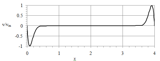
Figure 8 Profile of vertical velocity vvisualizes the boundary layers near the cold (at x = 0) and hot (at x = 4) sidewalls at y = 0.2826 and Gr_h = 104.

To find the limiting boundary-layer features, we plot in Figure 9 the v profile near the hot wall, using the scaled distance from the wall $\eta =0.482(L-x){\left(RaL\right)}^{1/4}$ , at Gr_h = 10³ (triangles), 10⁴ (squares), 10⁵ (circles) and 10⁶ (crosses). The symbols also show the grid points. The solid curve in Figure 9 depicts the analytical solution obtained by Gill²⁵ in the boundary layer approximation for a single-fluid flow near a hot wall,

$v/v_{max}=3.102exp(-\eta )sin\eta , \eta =0.482(L-x){\left(RaL\right)}^{1/4}$.                                (34)

Figure 9 Boundary-layer profile of vertical velocity vnear the hot wall at y = 0.2826 and Gr_h = 10³ (triangles), 10⁴ (squares), 10⁵ (circles) and 10⁶ (crosses). The solid curve depicts solution (34); $\eta =0.482(L-x){\left(RaL\right)}^{1/4}$ .

Figure 9 reveals that as Gr increases, the numerical results merge into the limiting profile which is rather close to analytical solution (34). Figure 9 shows both the jet-like character and the scale of boundary layer near the hot wall in the water domain. Thus as Gr increases, the water vertical motion becomes limited to thin vicinities of the container ends. This occurs due to stable stratification of water density.

Development of temperature boundary layers near sidewalls

Figure 10 shows the transformation of the temperature profile at the interface as the Grashof number Gr_h increases from 10² to 10⁸. At Gr_h = 102, the temperature distribution (solid line in Figure 10) is closed to that due to conduction only being nearly linear according to relation (2). For larger Gr_h, the thermal boundary layer develops first near the cold wall, x = 0, and then near the hot wall, x = 4. This sequence is physically reasonable since water moves from the hot end to the cold end along the interface. As Gr_h increases, this convection transports more heat and thus makes the temperature near the cold wall significantly larger than that provided by thermal conduction alone. Figure 10 illustrates this development near x = 0.

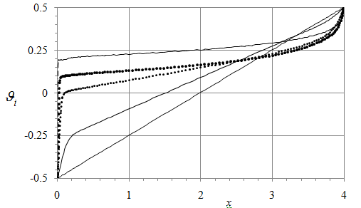
Figure 10 Distribution of temperature along the interface shows the formation of thermal boundary layer near cold, x = 0, and hot, x = 4, walls as Gr increases: Gr = 100 (solid line), 10⁴ (dashes), 10⁵ (small dots), 10⁶ (bold dots) and 10⁸ (dots and dashes).

Near the hot wall, the interface motion entrains the colder water from the depths thus decreasing the temperature below its conduction-alone value. Figure 10 illustrates this development near x = 4. Away from the end walls, the temperature remains to be a nearly linear function of x, but the $\partial \vartheta /\partial x$  value reduces as Gr_h increases, e.g., at x = 1 in Figure 10.

This change in the temperature distribution strengthens (weakens) the buoyancy effect near the vertical walls (in the bulk flow), that results in the development first the vertical jets discussed above and then jet-like boundary layers near the bottom and interface which are discussed below.

Development of boundary layers near horizontal boundaries

The experimental results for single-fluid flows^2,4 show that the boundary layers also develop near the horizontal walls as Gr increases. This development occurs for significantly larger Gr than those at which the jets form near the vertical walls. Figure 11 depicts the profile of the horizontal velocity u(y) at x = L/2 = 2 for Gr_h = 100 (curve) and 106 (dots). For convenient comparison of the results at these very different Gr_h values, the velocity is normalized by its magnitude (which is achieved at the interface), $u_i=\left|u\left(H_i\right)\right|$ where H_i = 0.5 here.

Figure 11 Vertical distribution of normalized horizontal velocity at x = L/2, H_i = 0.5 and Grh = 100 (curve) and 10^{6,/ (dots).}

Figure 11 shows that while the u-profiles are remarkably different in air, in water they are close for Gr_h = 100 and 106. The air-flow profile at Gr_h = 10⁶ agrees with the streamline pattern in Figure 7(b). The buoyancy driving dominates over the water driving that makes the air velocity maximal magnitude near the top wall close to the water velocity maximal magnitude near the bottom. This significant change practically does not affects the water velocity showing that the air impact on the water motion is negligible at H_i = 0.5. The water u-profile at Gr_h = 10⁶ is slightly shifted downward near the bottom compared with that at Gr_h = 100. This shift is a precursor of the boundary layer development near the bottom for larger Gr_h described below.

Figure 12 depicts the u-profiles in water only and reveals (a) the development of jet-like boundary layers near the bottom and near the interface and (b) the velocity reversal near the central stagnation point where u = 0. These flow features are similar to those observed in the experimental² and numerical ⁵ studies of single-fluid (water) convection in a horizontal container.

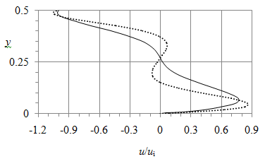
Figure 12 Vertical distribution of normalized horizontal velocity in water at x = L/2, H_i = 0.5 and Grh = 10⁷ (curve) and 10⁸ (dots).

Figure 13 depicts the profile of temperature at x = L/2 = 2 and Gr_h = 100 (curve), 10⁴ (dashes) and 10⁶ (dash-dotted curve) and 10⁸ (dots). Up to Gr_h = 10⁶, the temperature mostly varies in the water domain developing a strong stable density stratification as Gr_h increases. Note that as $G{r}_h\to \infty$ , the limiting values of the bottom (top) temperature is$\vartheta =-0.5\left(0.5\right)$ . At Gr_h = 10⁸, the vertical variation of temperature in air also becomes remarkable. This variation is due to the intensified thermal convection in the air domain as Table 1 illustrates. It shows that the characteristic Reynolds numbers of horizontal flow of water ( ${\left|u_h\right|}_{max}$ )and air (${\left|u_l\right|}_{max}$ ) are moderate even at Gr_h = 10⁷. It is interesting that ${\left|u_h\right|}_{max}>>{\left|u_l\right|}_{max}$  for $G{r}_h\le {10}^5$ , but ${\left|u_h\right|}_{max} <{\left|u_l\right|}_{max}atG{r}_h\ge {10}^6$ .

 Change in the water flow topology

Figure 13 Vertical distribution of temperature at x = L/2, H_i = 0.5 and Gr_h = 100 (solid bold line), 10⁴ (dashes) and 10⁶ (dash-dotted curve) and 10⁸ (dots).

Figure 14 depicts streamline pattern at Gr_h = 10⁸. The flow topology in Figure 14 differs with that shown in Figure 7(b) in both air and water domains. In Figure 7(b), the air flow has not only the global circulation near the domain boundary, but also the eight-figure pattern with a saddle stagnation point, connecting the internal circulation cells, and two centers within each of the cells. In contrast, the air flow is one-cellular in Figure 14. The water flow topology changes oppositely: it is one-cellular in Figure 7(b) while have the eight-figure pattern in Figure 14. The water pattern shown in Figure 14 is topologically identical to that experimentally observed in the single-fluid convection (Figure 6).⁴ The emergence of the eight-figure pattern in the water flow was numerically described and explained by the jet entrainment mechanism.⁵

Figure 14 (Color online) Streamline patterns at L = 4, H_i = 0.5, Ma = 0 and Gr_h = 10⁸.

Here in order to explore the thermal effect of the surface tension, we fix Gr = 10⁴, L = 4, = 0.5, and increase Ma.

Peaks of horizontal velocity near the sidewalls

Figure 15 depicts the horizontal velocity u(x) at the interface at Ma = 0 (dashed curve) 100 (solid curve) and 200 (dots). Since the velocity is negative being directed from the hot end to the cold end, we show -u for convenient presentation in Figure 15. As Ma increases, the velocity magnitude grows away from the sidewalls since the Marangoni stresses faster drive the water at the interface. A striking feature is that u-velocity peaks develop near the vertical walls as Ma increases.

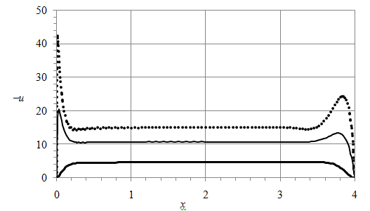
Figure 15 Velocity at the interface at Ma = 0 (dashes) 100 (solid curve) and 200 (dots); Gr_h = 10⁴, L = 4 and H_i = 0.5.

Temperature boundary layers near the sidewalls

To better understand physical mechanism of the velocity peak development, shown in Figure 15, we depict the temperature distribution along the interface in Figure 16. It shows the development of temperature boundary layers near the vertical walls. As Ma increases, $\partial \vartheta /\partial x$  slightly decreases away from the sidewalls, x = 0 and x = 4, while strongly grows near the sidewalls. The $\partial \vartheta /\partial x$  growth is especially remarkable near the cold wall because the water flow transports heat from the hot end to the cold end near the interface. This effect of increasing Ma is analogous to that of increasing Gr as comparison of Figure 10 & Figure 16 shows.

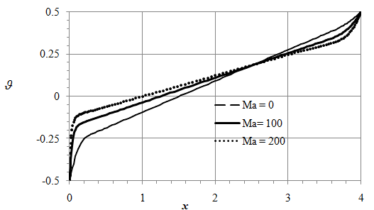
Figure 16 Temperature at the interface at Ma = 0 (dashed curve) and 100 (solid curve); Gr_h = 10⁴. L = 4 and H_i = 0.5.

Since the Marangoni shear stress is proportional to $\partial \vartheta /\partial x$  , the Marangoni driving focuses near x = 0 and x = L resulting in the u-velocity peaks shown in Figure 15. The temperature gradient is maximal near the cold wall, as Figure 16 illustrates, and accordingly the velocity peak near the cold end is larger than that near the hot end in Figure 15. Features of the velocity boundary layer near the cold wall are discussed below.

Velocity boundary layer near the cold end

Figure 17 depicts the dependence of the horizontal velocity on the interface, normalized by its minimal (maximal-magnitude) value, on the scaled distance from the cold sidewall, $\eta =xMa$ . The results for Ma = 100 and 200 in the scaled variables nearly merge in a single curve in Figure 17 thus revealing the boundary-layer shape and dimension. The velocity peak is located at the distance around x = x_m = 3.4/Ma from the cold wall and $|\partial u/\partial x|$  at x = 0 is proportional to Ma² that limits our numerical simulations to moderate Ma values (the symbols in Figure 17 also show the grid points).

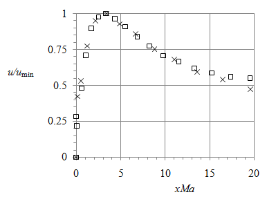
Figure 17 Merging of the results at Ma = 100 (squares) and 200 (crosses) shows the boundary-layer profile of normalized velocity at the interface near the cold sidewall.

Transformation of the air flow

As Ma increases, the water motion intensifies and drives the adjacent air flow. This results in the upward expansion of the air cell adjusted to the interface and the reduction of the air local cells as comparison shows of the streamline patterns at Ma = 0 in Figure 18(a) and at Ma = 200 in Figure 18(b).

Figure 18 (Color online) Transformation of flow pattern as Ma increases from 0 (a) to 200 (b).

First we check our stability code for the horizontal flow by comparison of our results with those in Table 2 in Reference²⁶ using the same mesh, 131x51, and parameter values, Pr = 6.78 and A_x = 2.5. Our simulations yields Re_cr1 = 1548 while Re_cr1 = 1430 in.²⁶ Using more grid points does not change our value of Re_cr1. We estimate this check-up as sufficient to the goal of this Section.

It follows from previous studies^9,11 that critical Gr is minimal at Pr = 0. This feature is physically reasonable because temperature variation typically results in the stable stratification of density. Therefore in order to ease the stability study, we multiply the Pr values for air and water by parameter b which varies from 0 to 1. We start with b = 0, where Pr = 0 for both fluids, and eventually increases b up to 1.

We found that at b = 0, Ma = 0 and H_i = 0.5, the critical parameters are: Gr = 4.75×10⁵, k = 0, $\alpha =2.88,{\omega }_r=-20.2,{\omega }_i=0,and{\left|u_h\right|}_{max}=287$ . Figure 19 depicts the base-flow velocity u_b(y) in the heavy (thin solid curve) and light (thin dots) fluid and the critical disturbance kinetic energy E_d(y) (bold curve and dots). Here $Ed=<{\left|u_d\right|}^2+{\left|v_d\left|{}^2+\right|w_d\right|}^2>$  where the brackets denote averaging with respect to time. Both u_b and E_d are normalized by their maximal magnitudes for convenient observation in one figure. Since E_d significantly drops as y increases from 0.5, the instability develops in the heavy-fluid flow. Figure 20 shows that the critical value of Gr grows as b increases. For b > 0.3, critical Gr is unbounded. This agrees with the previous results^9,11 that the shear-layer instability is suppressed as Pr increases. We conclude that the horizontal flow is stable at this Ma and H_i values.

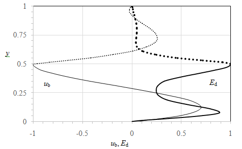
Figure 19 Profiles of base-flow velocity ub and disturbance kinetic energy E_d at critical Gr = 4.75×10⁵ at Pr = 0, Ma = 0 and H_i = 0.5.

Figure 20 Growth of critical Gr as Pr increases.

Here we first check our stability code for the two-dimensional convection by comparison of our results with those in Table 1 in Ref.²⁷ Our simulations yield Gr_cr = 2917647 for mesh 51 x 51 while Gr_cr = 2908327 in Ref.²⁷ We consider the agreement being satisfactory.

In the stability study of the two-dimensional convection, we fix L = 4 and H_i = 0.5 to be consistent with the results of Sections 9 and 10. Figure 21 depicts a typical spectrum of eigenvalues $\omega ={\omega }_r+i{\omega }_{i}atGr={10}^6$ and Ma = 0. The least decaying mode, corresponding to the maximal value of${\omega }_i$ , has ${\omega }_r=0$ , i.e., monotonically varies with time (no oscillation). This mode is two-dimensional, k = 0. Table 5 shows that the k = 0 mode corresponds to the maximal value of ${\omega }_i$ .

Table 2 shows the effect of increasing Gr at Ma = 0 and k = 0. These results look counterintuitive. The value of ${\omega }_i$ typically increases with the flow strength resulting in the development of instability. In contrast, ${\omega }_i$  decreases as Gr increases according Table 2. We interpret this paradoxical trend as a result of the stable density stratification which strengthens as Gr increases. Based on this trend, we do not increase Gr beyond 10⁶ in the stability studies. Table 3 shows the effect of increasing Ma at Gr = 10⁴ and k = 0. Here ${\omega }_i$  also decreases as Ma grows although this trend is weaker than that in the case of increasing Gr. The above stability results indicate that the convection flow, described in Sections 9 and 10, are stable.

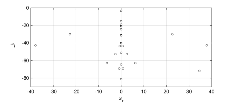
Figure 21 Spectrum of eigenvalues $\omega ={\omega }_r+i{\omega }_i$  at Gr = 10⁶ , Ma = 0 and k = 0.

The main result of this study is that the adiabatic horizontal walls make the air-water thermo-gravitational convection stable in the horizontally elongated container with lateral heating. To this end, we first show that the flow becomes nearly horizontal except in thin vicinities of the vertical walls.

A compact polynomial solution is obtained which describes the horizontal convection (Section 6). This solution explicitly shows how the number and profile of air and water counter-flows depend on (a) the water fraction, (b) the thermal surface-tension effect, characterized by the Marangoni number Ma, and (c) the buoyancy strength characterized by the Grashof number Gr.

Next, our numerical simulations describe the development of strong vertical jets in the boundary layers near the sidewalls. The numerical and analytical results agree away from the sidewalls for small and moderate Gr and Ma (Section 8) that verify both of them.

Then jet-like boundary layers develop near the horizontal walls as Gr (Section 9) and Ma (Section 10) increase. The jet entrainment generates two new cells between the boundary layers in the water flow (Section 9). As Ma increases, the Marangoni stresses focus near the sidewalls and develop a thin boundary layer near the cold end (Section 10).

The stability studies of the horizontal (Section 11) and two-dimensional (Section 12) flows reveal no instability of the steady convection described in Sections 6, 8, 9, and 10. The stability is achieved due to the adiabatic walls which provide the favorable stratification of water density. The effect of the air motion on the water flow is found negligible if the water volume fraction is not very small.

These results, related to the flow patterns and stability, agree with the experimental observations² and can be utilized for the development of efficient heat exchangers.

To check-up the grid-independence of our stability results, we consider two cases presented in Tables 6 & 7. The check-up demonstrates that the resolution is good enough providing the sufficiently accurate results for the flow stability features.

Partial support from the Ministry of Science and Education (Spain) through Grant No. DPI2016-78887 is gratefully acknowledged.

The authors declare that there is no conflict of interests regarding the publication of this paper.

References

1. Hart JE. On the influence of centrifugal buoyancy on rotating convection. J Fluid Mech. 2000;403:133‒151.
2. Kirdyashkin AG. Thermogravitational and thermocapillary flows in a horizontal temperature gradient. Int J Heat Mass Transfer. 1984;27:1205‒1218.
3. Daniels PG, Blythe PA, Simpkins PG. Onset of multicellular convection in a shallow laterally heated cavity. Proceedings of the Royal Society of London. 1987;411(1841):327‒350.
4. Bejan A, Al Homoud AA, Imberger J. Experimental study of high-Rayleigh number convection in a horizontal cavity with differentially end temperature. J Fluid Mech. 1981;109:283‒299.
5. Herrada MA, Shtern VN. Velocity reversals via bifurcation in thermal convection. Int J Heat Mass Transfer. 2016;92:66‒75.
6. Ostroumov GA. Free convection under the conditions of the internal problem. NACA TM No. 1407, National Advisory Committee for Aeronautics, USA; 1952. 233 p.
7. Birikh RV. Thermocapillary convection in a horizontal layer, of liquid. J Appl Mech Tech Phys. 1966;7(3):43‒44.
8. Nepomnyashchy A, Simanovskii I, Legros JC. Interfacial Convection in Multilayer Systems. 2nd Springer; 2012. 498 p..
9. Birikh RV. On small perturbations of a plane-parallel with a cubic velocity profile. J Appl Math Mech. 1967;30(2):432‒438.
10. Gershuni GZ, Zhukhovitsky EM, Myznikov VM. Stability of a plane-parallel convective flow of a liquid in a horizontal layer. J Appl Mech Tech Phys. 1974;15(1):78‒82.
11. Gershuni GZ, Zhukhovitsky EM, Myznikov VM. Stability of plane-parallel convective flow in a horizontal layer relative to spatial perturbations. J Appl Mech Tech Phys. 1974;15(5):706‒708.
12. Herrada MA, Shtern VN. Stability of centrifugal convection in a rotating pipe. Phys Fluids. 2015;27(6):064106.
13. Shtern V, Zimin V, Hussain F. Analysis of centrifugal convection in rotating pipes. Phys Fluids. 2001;13(8):2296‒2308.
14. Birikh RV, Pukhnachev VV. An axial convective flow in a rotating tube with a longitudinal temperature gradient. Doklady Physics. 2011;56(1):47‒52.
15. Herrada MA, Shtern VN. Air-water centrifugal convection. Phys Fluids. 2014;26(7):072102.
16. Madruga S, Pérez-García C, Lebon G. Convective instabilities in two superposed horizontal liquid layers heated laterally. Phys Rev E. 2003;68:041607.
17. Sparrow EM, Azevedo LFA, Prata AT. Two-fluid and single-fluid natural convection heat transfer in an enclosure. J Heat Transfer. 1986;108(4):848‒852.
18. Villers D, Platten JK. Thermal convection in superposed immiscible liquid layers. Appl Sci Res. 1988;45(2):145‒152.
19. Villers D. Platten JK. Influence of interfacial tension gradients on thermal convection in two superposed immiscible liquid layers. Appl Sci Res. 1990;47(2):177‒191.
20. Doi T, Koster JN. Thermocapillary convection in two immiscible liquid layers with free surface. Phys Fluids A. 1993;5(8):1914‒1927.
21. Liu QS, Chen G, Roux B. Thermogravitational and thermocapillary convection in a cavity containing two superposed immiscible liquid layers. Int J Heat Mass Transfer. 1993;36:101‒117.
22. Liu QS, Roux B, Velarde MG. Thermocapillary convection in two-layer systems. Int J Heat Mass Transfer. 1998;41:1499‒1511.
23. Herrada MA, Montanero JM. A numerical method to study the dynamics of capillary fluid systems. J of Comput Phys. 2016;306:137‒147.
24. Herrada MA, Shtern VN. Instability of water-spout problem. Phys Fluids. 2016;28:034107.
25. Gill AE. The boundary-layer regime for convection in a rectangular cavity. J Fluid Mech. 1966;26(3):515‒536.
26. Xu J, Zebib A. Oscillatory two- and three-dimensional thermocapillary convection. J Fluid Mech. 1998;364:187‒209.
27. Gelfgat A. Stability of convective flows in cavities: Solution of benchmark problems by a low-order finite volume method. Int J Numer Mech Fluids. 2007;53(3):485‒506.
Creative Commons Attribution License
©2017 Herrada, et al. This is an open access article distributed under the terms of the, which permits unrestricted use, distribution, and build upon your work non-commercially.