Submit manuscript...
eISSN: 2378-315X

Biometrics & Biostatistics International Journal

Research Article Volume 5 Issue 3

Using the ROC curve to measure association and evaluate Prediction accuracy for a binary outcome

Jingjing Yin, Robert L Vogel

Department of Biostatistics, Jiann-Ping Hsu College of Public Health, Georgia Southern University, USA

Correspondence: Jingjing Yin, Department of Biostatistics, Jiann-Ping Hsu College of Public Health, Georgia Southern University, USA

Received: January 30, 2016 | Published: March 15, 2017

Citation: Yin J, Vogel RL. Using the roc curve to measure association and evaluate prediction accuracy for a binary outcome. Biom Biostat Int J. 2017;5(3):95-103. DOI: 10.15406/bbij.2017.05.00134

Download PDF

Abstract

This review article addresses the ROC curve and its advantage over the odds ratio to measure the association between a continuous variable and a binary outcome. A simple parametric model under the normality assumption and the method of Box-Cox transformation for non-normal data are discussed. Applications of the binormal model and the Box-Cox transformation under both univariate and multivariate inference are illustrated by a comprehensive data analysis tutorial. Finally, a summary and recommendations are given as to the usage of the binormal ROC curve.

Keywords: odds ratio, box-cox transformation, binormal ROC, AUC, youden index

Introducton

Logistic regression and its corresponding odds ratio(s) (OR) are the most popular measure of association between a continuous or categorical variable with a binary outcome in epidemiology. For example, in epidemeology, we would be interested in the association between health status and life style measures. For a significantly associated predictor of a binary outcome, we can estimate the probability of a random observation being in one category and classify the observation into two groups based on the value of the predictor. For example, it is believed that arsenic exposure is associated with blackfoot disease. Such exposure can be continuous, i.e., the level of chronic arsenic exposure through drinking water, or binary, i.e., exposed versus non-exposed. However, using logistic regression and the odds ratio sometimes produces results that are puzzling and misleading: Kraemer and Pepe et al.1,2 provided very good discussions about the paradoxical situations about the odds ratio, especially in the presence of strongly associated predictors.

The odds ratio is the ratio between the odds of an outcome event of interest in one category of the predictor variable versus the odds of the same event in the other category of the predictor. For example, the odds ratio of arsenic exposure for blackfoot disease is defined as the ratio between the odds of getting the blackfoot disease in the exposed group versus the odds in the non-exposed group. Commonly, a variable associated with a binary outcome is interpreted as a rule for classification or prediction of the binary outcome. In order to predict or classify subjects into two categories, a cut-off point/threshold is needed if the predictor is continuous. Similarly, if the predictor is categorical with more than two levels, then a grouping of neighboring categories is needed. For example, in the field of medical diagnostics, some continuous biomarkers that are associated with the disease outcome are used to identify the sub-clinical diseased individuals. In medical diagnostics, it is common to assume that the diseased subject generally has a larger biomarker value than the healthy subject. In practice, sometimes a transformation of the biomarker values is necessary in order to meet such assumption. For example, HIV patients generally have lower CD4 cell counts, so we can transform the biomarker values as the reciprocal of the CD4 cell counts. An individual receives a positive diagnosis if his/her biomarker value of the diagnostic test is greater than the threshold; otherwise the diagnosis is considered “negative". Generally, physicians determine the true disease status by the long-established reference standard, which is sometimes called the “gold standard". Finally, for evaluation of the prediction accuracy of a biomarker/diagnostic test for the true disease status, a two-by-two association table is formed as in Table 1.


Reference standard


Diseased

Healthy

Diagnostic

Positive

TP

FP

test result

Negative

FN

TN

Table 1 Contingency table of reference standard versus diagnostic test result

 TP, true positive; TN, true negative; FP, false positive; FN, false negative

In practice, the diseased and the healthy population distributions generally overlap, which means there exist diagnostic errors. The false negative (FN) is “those who have disease and are diagnosed as negative" and the false positive (FP) is “those who do not have disease and are diagnosed as positive". The corresponding correct cases are the true positive (TP) and the true negative (TN), which are “those who have disease and are diagnosed as positive" and “those who do not have disease and are diagnosed as negative", respectively. The proportion of true positives among the diseased population is commonly referred as the sensitivity and the proportion of true negatives among the healthy population as the specificity. The sensitivity and specificity characterize the diagnostic accuracy under the diseased and the healthy populations, respectively. Mathematically, the sensitivity and specificity are

Specificity= TP TP+FN MathType@MTEF@5@5@+= feaagKart1ev2aaatCvAUfeBSjuyZL2yd9gzLbvyNv2CaerbuLwBLn hiov2DGi1BTfMBaeXatLxBI9gBaerbd9wDYLwzYbItLDharqqtubsr 4rNCHbGeaGqkY=xjYJH8sqFD0xXdHaVhbbf9v8qqaqFr0xc9pk0xbb a9q8WqFfeaY=biLkVcLq=JHqpepeea0=as0Fb9pgeaYRXxe9vr0=vr 0=vqpWqaaeaabiGaciaacaqabeaadaqaaqaaaOqaaKqzGeGaam4uai aadchacaWGLbGaam4yaiaadMgacaWGMbGaamyAaiaadogacaWGPbGa amiDaiaadMhacqGH9aqpkmaalaaajuaGbaqcLbsacaWGubGaamiuaa qcfayaaKqzGeGaamivaiaadcfacqGHRaWkcaWGgbGaamOtaaaaaaa@4C32@

Specificity= TP TN+FP MathType@MTEF@5@5@+= feaagKart1ev2aaatCvAUfeBSjuyZL2yd9gzLbvyNv2CaerbuLwBLn hiov2DGi1BTfMBaeXatLxBI9gBaerbd9wDYLwzYbItLDharqqtubsr 4rNCHbGeaGqkY=xjYJH8sqFD0xXdHaVhbbf9v8qqaqFr0xc9pk0xbb a9q8WqFfeaY=biLkVcLq=JHqpepeea0=as0Fb9pgeaYRXxe9vr0=vr 0=vqpWqaaeaabiGaciaacaqabeaadaqaaqaaaOqaaKqzGeGaam4uai aadchacaWGLbGaam4yaiaadMgacaWGMbGaamyAaiaadogacaWGPbGa amiDaiaadMhacqGH9aqpkmaalaaajuaGbaqcLbsacaWGubGaamiuaa qcfayaaKqzGeGaamivaiaad6eacqGHRaWkcaWGgbGaamiuaaaaaaa@4C32@

The odds ratio in medical diagnostic setting is referred as the diagnostic odds ratio (DOR), which is defined as the ratio of the odds of a positive result of a diagnostic test in the diseased population relative to that in the non-diseased population.3 Equivalently, the DOR is the ratio of the odds of the disease among the test positives versus that in the test negatives:

DOR= TP/FN FP/TN = TP/FP FN/TN = sensitivity specificity ( 1sensitivity )( 1specificity ) MathType@MTEF@5@5@+= feaagKart1ev2aaatCvAUfeBSjuyZL2yd9gzLbvyNv2CaerbuLwBLn hiov2DGi1BTfMBaeXatLxBI9gBaerbd9wDYLwzYbItLDharqqtubsr 4rNCHbGeaGqkY=xjYJH8sqFD0xXdHaVhbbf9v8qqaqFr0xc9pk0xbb a9q8WqFfeaY=biLkVcLq=JHqpepeea0=as0Fb9pgeaYRXxe9vr0=vr 0=vqpWqaaeaabiGaciaacaqabeaadaqaaqaaaOqaaKqzGeGaamirai aad+eacaWGsbGaeyypa0JcdaWcaaqcfayaaKqzGeGaamivaiaadcfa caGGVaGaamOraiaad6eaaKqbagaajugibiaadAeacaWGqbGaai4lai aadsfacaWGobaaaiabg2da9OWaaSaaaKqbagaajugibiaadsfacaWG qbGaai4laiaadAeacaWGqbaajuaGbaqcLbsacaWGgbGaamOtaiaac+ cacaWGubGaamOtaaaacqGH9aqpkmaalaaajuaGbaqcLbsacaWGZbGa amyzaiaad6gacaWGZbGaamyAaiaadshacaWGPbGaamODaiaadMgaca WG0bGaamyEaabaaaaaaaaapeGaaiiOaiaadohacaWGWbGaamyzaiaa dogacaWGPbGaamOzaiaadMgacaWGJbGaamyAaiaadshacaWG5baaju aGpaqaaOWaaeWaaKqbagaajugibiaaigdacqGHsislcaWGZbGaamyz aiaad6gacaWGZbGaamyAaiaadshacaWGPbGaamODaiaadMgacaWG0b GaamyEaaqcfaOaayjkaiaawMcaaOWaaeWaaKqbagaajugibiaaigda cqGHsislcaWGZbWdbiaadchacaWGLbGaam4yaiaadMgacaWGMbGaam yAaiaadogacaWGPbGaamiDaiaadMhaaKqba+aacaGLOaGaayzkaaaa aaaa@89A0@

Generally, an odds ratio of 1 indicates no association between the predictor and the outcome. Therefore, a DOR=1 means that the diagnostic test does not discriminate better than random chance between the diseased patients and those without the disease. The DOR rises steeply when one of the pair (sensitivity, specificity) becomes nearly perfect, while the other one of the pair may stay unsatisfactory. For example, when sensitivity=0.99 MathType@MTEF@5@5@+= feaagKart1ev2aaatCvAUfeBSjuyZL2yd9gzLbvyNv2CaerbuLwBLn hiov2DGi1BTfMBaeXatLxBI9gBaerbd9wDYLwzYbItLDharqqtubsr 4rNCHbGeaGqkY=xjYJH8sqFD0xXdHaVhbbf9v8qqaqFr0xc9pk0xbb a9q8WqFfeaY=biLkVcLq=JHqpepeea0=as0Fb9pgeaYRXxe9vr0=vr 0=vqpWqaaeaabiGaciaacaqabeaadaqaaqaaaOqaaKqzGeaeaaaaaa aaa8qacaWGZbGaamyzaiaad6gacaWGZbGaamyAaiaadshacaWGPbGa amODaiaadMgacaWG0bGaamyEaiabg2da9iaaicdacaGGUaGaaGyoai aaiMdaaaa@4763@ and specificity=0.5 MathType@MTEF@5@5@+= feaagKart1ev2aaatCvAUfeBSjuyZL2yd9gzLbvyNv2CaerbuLwBLn hiov2DGi1BTfMBaeXatLxBI9gBaerbd9wDYLwzYbItLDharqqtubsr 4rNCHbGeaGqkY=xjYJH8sqFD0xXdHaVhbbf9v8qqaqFr0xc9pk0xbb a9q8WqFfeaY=biLkVcLq=JHqpepeea0=as0Fb9pgeaYRXxe9vr0=vr 0=vqpWqaaeaabiGaciaacaqabeaadaqaaqaaaOqaaKqzGeaeaaaaaa aaa8qacaWGZbGaamiCaiaadwgacaWGJbGaamyAaiaadAgacaWGPbGa am4yaiaadMgacaWG0bGaamyEaiabg2da9iaaicdacaGGUaGaaGynaa aa@466D@ , DOR=99 MathType@MTEF@5@5@+= feaagKart1ev2aaatCvAUfeBSjuyZL2yd9gzLbvyNv2CaerbuLwBLn hiov2DGi1BTfMBaeXatLxBI9gBaerbd9wDYLwzYbItLDharqqtubsr 4rNCHbGeaGqkY=xjYJH8sqFD0xXdHaVhbbf9v8qqaqFr0xc9pk0xbb a9q8WqFfeaY=biLkVcLq=JHqpepeea0=as0Fb9pgeaYRXxe9vr0=vr 0=vqpWqaaeaabiGaciaacaqabeaadaqaaqaaaOqaaKqzGeaeaaaaaa aaa8qacaWGebGaam4taiaadkfacqGH9aqpcaaI5aGaaGyoaaaa@3DE9@ . However, the total correct classification rate is sensitivity+specificity=1.49 MathType@MTEF@5@5@+= feaagKart1ev2aaatCvAUfeBSjuyZL2yd9gzLbvyNv2CaerbuLwBLn hiov2DGi1BTfMBaeXatLxBI9gBaerbd9wDYLwzYbItLDharqqtubsr 4rNCHbGeaGqkY=xjYJH8sqFD0xXdHaVhbbf9v8qqaqFr0xc9pk0xbb a9q8WqFfeaY=biLkVcLq=JHqpepeea0=as0Fb9pgeaYRXxe9vr0=vr 0=vqpWqaaeaabiGaciaacaqabeaadaqaaqaaaOqaaKqzGeaeaaaaaa aaa8qacaWGZbGaamyzaiaad6gacaWGZbGaamyAaiaadshacaWGPbGa amODaiaadMgacaWG0bGaamyEaiabgUcaRiaadohacaWGWbGaamyzai aadogacaWGPbGaamOzaiaadMgacaWGJbGaamyAaiaadshacaWG5bGa eyypa0JaaGymaiaac6cacaaI0aGaaGyoaaaa@5294@  which indicates a moderate predictor for diagnosis. Furthermore, a large value of the DOR sometimes have very wide confidence intervals. Additionally, for a continuous predictor, in order to make a prediction or a classification for a binary outcome, a cut-off point or threshold value is needed which is usually estimated by some optimization criteria. Bohning et al.4 found that determining an optimal cut-off value via maximizing the DOR might lead to optimal cut-off estimates on the boundary of the parameter range, which clearly is not an “optimal" cut-off value to use for classification. In summary, a predictor with a large DOR does not necessarily yield good prediction. Therefore, we need alternative approaches for evaluating associations. In this paper, we recommend the use of the Receiver Operating Characteristic (ROC) curve.

In the following, we introduce the basics of the ROC curve and its summary indices in section 2. Section 3 present a parametric approach for making inference for the ROC analysis using binormal model under the assumption of binormality (i.e., both the diseased and healthy populations are normally distributed). In section 4, we discuss the use of the Box-Cox transformation for non-normally distributed data. Section 5 illustrates the binormal ROC analysis using a real data set. Finally we give a summary and discussion in section 6.

Basics about the ROC curve

For a continuous predictor, at each of the pre-specified threshold values, paired values of sensitivity and specificity can be computed. The Receiver Operating Characteristic (ROC) curve is a graph plotting the pair of (1− specificity, sensitivity) for all possible threshold values. Therefore, this graph demonstrates a trade-off phenomena between sensitivity and specificity. The ROC curve is an important and popular tool for the evaluation of the diagnostic tests. It can be used to demonstrate associations between a continuous variable for a binary outcome, as well as help to evaluate the accuracy of the prediction and classification based on a continuous variable. Extensive statistical research has been done in this field and there are several excellent reviews of statistical methods involving ROC curves.58

In theory, the ROC curve of a perfect diagnostic test would be the one connecting points (0,0), (0,1) and (1,1). The point (0,1) is sometimes referred as the perfection point. Some practitioners may compare different diagnostic tests for the same disease based on visual inspection of the estimated ROC curves that do not overlap. The optimal test is the one with the ROC curve bending most towards the perfection point. However, this is not applicable for situations when the fitted ROC curves cross each other, which frequently occurs in practice. Furthermore, even if the fitted ROC curves do not overlap, due to sampling variability, such visual inspection of the estimated ROC curves is still not a valid approach to make formal comparisons between tests. Therefore, there is a need for some type of formal index to summarize the ROC curve. Among all summary measures of the ROC curve, the area under the ROC curve (AUC) is very popular.

The AUC can be calculated by the integration of the ROC curve with respect to the false positive rate over [0,1]. The AUC is an overall summary of the ROC curve across all thresholds which is invariant to the prevalence of the disease and the choice of the diagnostic threshold. Under the assumption that a larger biomarker value indicates greater likelihood of the disease, Bamber and Donald8 showed that the AUC equals the probability of the marker value D of a randomly selected subject from the diseased population being greater than the marker value H of a randomly selected subject from the healthy population. This is denoted as AUC=Pr( D>H ) MathType@MTEF@5@5@+= feaagKart1ev2aaatCvAUfeBSjuyZL2yd9gzLbvyNv2CaerbuLwBLn hiov2DGi1BTfMBaeXatLxBI9gBaerbd9wDYLwzYbItLDharqqtubsr 4rNCHbGeaGqkY=xjYJH8sqFD0xXdHaVhbbf9v8qqaqFr0xc9pk0xbb a9q8WqFfeaY=biLkVcLq=JHqpepeea0=as0Fb9pgeaYRXxe9vr0=vr 0=vqpWqaaeaabiGaciaacaqabeaadaqaaqaaaOqaaKqzGeaeaaaaaa aaa8qacaWGbbGaamyvaiaadoeacqGH9aqpcaWGqbGaamOCaOWdamaa bmaabaqcLbsapeGaamiraiabg6da+iaadIeaaOWdaiaawIcacaGLPa aaaaa@431B@ . The AUC is more useful for evaluating a diagnostic test at early stages, for which the primary purpose is to pick up candidate tests with discriminating potentials. However, as a single index, the AUC lacks details about the trade-off between sensitivity and specificity, hence it cannot measure and balance the respective cost of the false positives and the false negatives. For different types of disease, the clinical-meaningful range of the sensitivity and specificity would vary. Therefore, the partial area under the ROC curve ( pAUC ) MathType@MTEF@5@5@+= feaagKart1ev2aaatCvAUfeBSjuyZL2yd9gzLbvyNv2CaerbuLwBLn hiov2DGi1BTfMBaeXatLxBI9gBaerbd9wDYLwzYbItLDharqqtubsr 4rNCHbGeaGqkY=xjYJH8sqFD0xXdHaVhbbf9v8qqaqFr0xc9pk0xbb a9q8WqFfeaY=biLkVcLq=JHqpepeea0=as0Fb9pgeaYRXxe9vr0=vr 0=vqpWqaaeaabiGaciaacaqabeaadaqaaqaaaOqaamaabmaabaqcLb saqaaaaaaaaaWdbiaadchacaWGbbGaamyvaiaadoeaaOWdaiaawIca caGLPaaaaaa@3DE8@ , which is obtained by integrating the ROC curve over a predetermined range of the false positive rate, would be more appropriate than the AUC for this purpose. Alternatively, sensitivity at a predetermined false positive rate can be used for specific applications.

For the purpose of making a diagnosis, a diagnostic threshold for the test is required. As the AUC is a global summary measure across all possible thresholds, separate computation after the AUC evaluation is needed to derive the optimal cut-off point for making diagnosis. Furthermore, the global measure AUC lacks direct link to the sensitivity and specificity, hence it is rather abstract for clinicians to understand and compute. For selecting an “optimal” diagnostic cut-off point, there exist a variety of approaches.10,11 Among them, the Youden index J MathType@MTEF@5@5@+= feaagKart1ev2aaatCvAUfeBSjuyZL2yd9gzLbvyNv2CaerbuLwBLn hiov2DGi1BTfMBaeXatLxBI9gBaerbd9wDYLwzYbItLDharqqtubsr 4rNCHbGeaGqkY=xjYJH8sqFD0xXdHaVhbbf9v8qqaqFr0xc9pk0xbb a9q8WqFfeaY=biLkVcLq=JHqpepeea0=as0Fb9pgeaYRXxe9vr0=vr 0=vqpWqaaeaabiGaciaacaqabeaadaqaaqaaaOqaaKqzGeaeaaaaaa aaa8qacaWGkbaaaa@39B8@ , defined as max c { sensitivity( c )+specificity( c )1 } MathType@MTEF@5@5@+= feaagKart1ev2aaatCvAUfeBSjuyZL2yd9gzLbvyNv2CaerbuLwBLn hiov2DGi1BTfMBaeXatLxBI9gBaerbd9wDYLwzYbItLDharqqtubsr 4rNCHbGeaGqkY=xjYJH8sqFD0xXdHaVhbbf9v8qqaqFr0xc9pk0xbb a9q8WqFfeaY=biLkVcLq=JHqpepeea0=as0Fb9pgeaYRXxe9vr0=vr 0=vqpWqaaeaabiGaciaacaqabeaadaqaaqaaaOqaaKqzGeGaciyBai aacggacaGG4bGcdaWgaaqcfasaaKqzGeGaam4yaaqcfayabaGcdaGa daqcfayaaKqzGeaeaaaaaaaaa8qacaGGZbWdaiaadwgacaWGUbGaam 4CaiaadMgacaWG0bGaamyAaiaadAhacaWGPbGaamiDaiaadMhakmaa bmaajuaGbaqcLbsacaWGJbaajuaGcaGLOaGaayzkaaqcLbsacqGHRa WkcaWGZbGaamiCaiaadwgacaWGJbGaamyAaiaadAgacaWGPbGaam4y aiaadMgacaWG0bGaamyEaOWaaeWaaKqbagaajugibiaadogaaKqbak aawIcacaGLPaaajugibiabgkHiTiaaigdaaKqbakaawUhacaGL9baa aaa@62D8@ , is very popular since it ties nicely into the ROC framework and it has a closed-form solution under normality.12 The cut-off point determined via the Youden index maximizes the overall correct classification rate (i.e., sum of sensitivity and specificity) and assigns equal weight to the sensitivity and the specificity. The Youden index has a clinical interpretation as a direct measure of the maximum diagnostic accuracy that a marker can achieve. Another advantage of the Youden index over the AUC is that it can detect differences other than in location while the AUC can only detect location differences between the diseased and healthy samples13 Graphically, the Youden index is the maximum vertical distance between the ROC curve and the chance line. It measures the difference of the diagnostic accuracy of a marker and that determined by random chance. In order to give varying weights for sensitivity and specificity, the weighted Youden index was proposed14,15 and is expressed as max c { W*sensitivity( c )+( 1W )*specificity( c )1 } MathType@MTEF@5@5@+= feaagKart1ev2aaatCvAUfeBSjuyZL2yd9gzLbvyNv2CaerbuLwBLn hiov2DGi1BTfMBaeXatLxBI9gBaerbd9wDYLwzYbItLDharqqtubsr 4rNCHbGeaGqkY=xjYJH8sqFD0xXdHaVhbbf9v8qqaqFr0xc9pk0xbb a9q8WqFfeaY=biLkVcLq=JHqpepeea0=as0Fb9pgeaYRXxe9vr0=vr 0=vqpWqaaeaabiGaciaacaqabeaadaqaaqaaaOqaaKqzGeGaciyBai aacggacaGG4bGcdaWgaaqcfasaaKqzGeGaam4yaaqcfayabaGcdaGa daqcfayaaKqzGeGaam4vaiaacQcaqaaaaaaaaaWdbiaacohapaGaam yzaiaad6gacaWGZbGaamyAaiaadshacaWGPbGaamODaiaadMgacaWG 0bGaamyEaOWaaeWaaKqbagaajugibiaadogaaKqbakaawIcacaGLPa aajugibiabgUcaROWaaeWaaKqbagaajugibiaaigdacqGHsislcaWG xbaajuaGcaGLOaGaayzkaaqcLbsacaGGQaGaam4CaiaadchacaWGLb Gaam4yaiaadMgacaWGMbGaamyAaiaadogacaWGPbGaamiDaiaadMha kmaabmaajuaGbaqcLbsacaWGJbaajuaGcaGLOaGaayzkaaqcLbsacq GHsislcaaIXaaajuaGcaGL7bGaayzFaaaaaa@6B61@  with predetermined weights W MathType@MTEF@5@5@+= feaagKart1ev2aaatCvAUfeBSjuyZL2yd9gzLbvyNv2CaerbuLwBLn hiov2DGi1BTfMBaeXatLxBI9gBaerbd9wDYLwzYbItLDharqqtubsr 4rNCHbGeaGqkY=xjYJH8sqFD0xXdHaVhbbf9v8qqaqFr0xc9pk0xbb a9q8WqFfeaY=biLkVcLq=JHqpepeea0=as0Fb9pgeaYRXxe9vr0=vr 0=vqpWqaaeaabiGaciaacaqabeaadaqaaqaaaOqaaKqzGeGaam4vaa aa@39A5@ and 1W MathType@MTEF@5@5@+= feaagKart1ev2aaatCvAUfeBSjuyZL2yd9gzLbvyNv2CaerbuLwBLn hiov2DGi1BTfMBaeXatLxBI9gBaerbd9wDYLwzYbItLDharqqtubsr 4rNCHbGeaGqkY=xjYJH8sqFD0xXdHaVhbbf9v8qqaqFr0xc9pk0xbb a9q8WqFfeaY=biLkVcLq=JHqpepeea0=as0Fb9pgeaYRXxe9vr0=vr 0=vqpWqaaeaabiGaciaacaqabeaadaqaaqaaaOqaaKqzGeGaaGymai abgkHiTiaadEfaaaa@3B4D@ .

Binormal model for ROC analysis

For the ROC analysis, sometimes, parametric assumptions are made on the distributions of the marker measurements for both healthy and diseased groups. The binormality assumption is the most popular as it utilizes many properties of the normal distribution and hence is the most straightforward for applications in practice. When the two discriminating populations are normally distributed or can be simultaneously transformed to normal after some monotonic transformation, the corresponding ROC curve satisfies the binormality assumption and is thus called the binormal ROC curve.1618 Hanley19 listed some primary justifications of applying the binormal model for fitting the ROC curves. These includes “Gaussian distribution is natural for many situations", “Other distributions can be approximated by Gaussian", “The ROC curve is invariant under monotonic transformation of marker values" and “Mathematical convenience based on nice properties of normality." The binormal ROC model provides a basis for parametric estimation and inference about the ROC curve and its summary indices. The binormal model generally fits well for continuous marker values. It is also robust for rating data on an ordinal scale assuming a continuous latent variable under large sample assumption.19 This article focuses on the binormal model fitted explicitly on the continuous biomarker values.

For making inference about the ROC curve using the binormal model, Linnet20 developed a parametric approach based on maximum likelihood estimation for sensitivity given a fixed value of specificity or false positive rate. The confidence interval about sensitivity at a single value of specificity or false positive rate can also be considered as the pointwise confidence interval for the ROC curve. For making inference about the whole or partial ROC curve and maintaining the type I error within the range of specificity, the simultaneous confidence band needs to be estimated. Ma and Hall21 proposed a parametric confidence band of the ROC curve by applying the binormal model and extending the Working and Hotelling22 confidence band for a regression line. Demidenko23 proposed an ellipse-envelope confidence band under binormality for the ROC curve. Yin and Tian24 proposed a generalized inference confidence band for the ROC Curve.

For the Youden index and its associated optimal cut-point, some researchers examined different estimation and inference methods under binormal assumption. For example, Fluss et al.25 compared parametric methods with and without the Box-Cox transformation; Schisterman and Perkins12 proposed asymptotic confidence intervals based on bi-normal and bi-gamma models; Lai and Tian26 applied the generalized inference method. For making inference about the AUC using the binormal model, Wieand et al.27 applied the delta method based asymptotic results to construct a test of difference between two AUCs in a paired design. Molodianovitch et al.28 applied the Box-Cox transformation for non-normal data and then applied the method of Wieand et al.27 on the transformed data. Tian29 and Li et al.30 applied the generalized pivotal quantity approach to obtain the exact confidence intervals for single AUC and paired AUC respectively. Recently, the parametric joint inference under binormality for two or more ROC summary indices were proposed. For example, Yin and Tian30 proposed joint confidence region estimation of the AUC and the Youden index based on the asymptotic delta method and generalized inference approach. Yin and Tian31 and Bantis et al.32 used similar approaches for joint inference about sensitivity and specificity at the optimal threshold value associated with the Youden index.

Under binormality

Let Y 1 Normal( μ 1 , σ 1 2 ) MathType@MTEF@5@5@+= feaagKart1ev2aaatCvAUfeBSjuyZL2yd9gzLbvyNv2CaerbuLwBLn hiov2DGi1BTfMBaeXatLxBI9gBaerbd9wDYLwzYbItLDharqqtubsr 4rNCHbGeaGqkY=xjYJH8sqFD0xXdHaVhbbf9v8qqaqFr0xc9pk0xbb a9q8WqFfeaY=biLkVcLq=JHqpepeea0=as0Fb9pgeaYRXxe9vr0=vr 0=vqpWqaaeaabiGaciaacaqabeaadaqaaqaaaOqaaKqzGeGaamywaO WaaSbaaKazfa4=baqcLbmacaaIXaaajuaGbeaajugibiablYJi6iaa d6eacaWGVbGaamOCaiaad2gacaWGHbGaamiBaOWaaeWaaKqbagaaju gibiabeY7aTPWaaSbaaKazfa4=baqcLbmacaaIXaaajuaGbeaajugi biaacYcacqaHdpWCkmaaDaaajqwba+FaaKqzadGaaGymaaqcKvaG=h aajugWaiaaikdaaaaajuaGcaGLOaGaayzkaaaaaa@59E3@  and Y 2 Normal( μ 2 , σ 2 2 ) MathType@MTEF@5@5@+= feaagKart1ev2aaatCvAUfeBSjuyZL2yd9gzLbvyNv2CaerbuLwBLn hiov2DGi1BTfMBaeXatLxBI9gBaerbd9wDYLwzYbItLDharqqtubsr 4rNCHbGeaGqkY=xjYJH8sqFD0xXdHaVhbbf9v8qqaqFr0xc9pk0xbb a9q8WqFfeaY=biLkVcLq=JHqpepeea0=as0Fb9pgeaYRXxe9vr0=vr 0=vqpWqaaeaabiGaciaacaqabeaadaqaaqaaaOqaaKqzGeGaamywaK qbaoaaBaaajuaibaqcLbmacaaIYaaajuaGbeaajugibiablYJi6iaa d6eacaWGVbGaamOCaiaad2gacaWGHbGaamiBaOWaaeWaaKqbagaaju gibiabeY7aTPWaaSbaaKqbGeaajugWaiaaikdaaKqbagqaaKqzGeGa aiilaiabeo8aZLqbaoaaDaaajuaibaqcLbmacaaIYaaajuaibaqcLb macaaIYaaaaaqcfaOaayjkaiaawMcaaaaa@53E2@  denote diagnostic marker measurements for the diseased and the healthy populations respectively. The cumulative distribution function (cdf) for the two populations is denoted as F Y i ( t )=Φ ( t μ i ) σ i MathType@MTEF@5@5@+= feaagKart1ev2aaatCvAUfeBSjuyZL2yd9gzLbvyNv2CaerbuLwBLn hiov2DGi1BTfMBaeXatLxBI9gBaerbd9wDYLwzYbItLDharqqtubsr 4rNCHbGeaGqkY=xjYJH8sqFD0xXdHaVhbbf9v8qqaqFr0xc9pk0xbb a9q8WqFfeaY=biLkVcLq=JHqpepeea0=as0Fb9pgeaYRXxe9vr0=vr 0=vqpWqaaeaabiGaciaacaqabeaadaqaaqaaaOqaaKqzGeGaamOraO WaaSbaaKqbagaajugWaiaadMfakmaaBaaajuaGbaqcLbsacaWGPbaa juaGbeaaaeqaaOWaaeWaaKqbagaajugibiaadshaaKqbakaawIcaca GLPaaajugibiabg2da9iabfA6agPWaaSaaaKqbagaakmaabmaajuaG baqcLbsacaWG0bGaeyOeI0IaeqiVd0wcfa4aaSbaaeaajugWaiaadM gaaKqbagqaaaGaayjkaiaawMcaaaqaaKqzGeGaeq4Wdmxcfa4aaSba aeaajugWaiaadMgaaKqbagqaaaaaaaa@565B@  for i=1,2 MathType@MTEF@5@5@+= feaagKart1ev2aaatCvAUfeBSjuyZL2yd9gzLbvyNv2CaerbuLwBLn hiov2DGi1BTfMBaeXatLxBI9gBaerbd9wDYLwzYbItLDharqqtubsr 4rNCHbGeaGqkY=xjYJH8sqFD0xXdHaVhbbf9v8qqaqFr0xc9pk0xbb a9q8WqFfeaY=biLkVcLq=JHqpepeea0=as0Fb9pgeaYRXxe9vr0=vr 0=vqpWqaaeaabiGaciaacaqabeaadaqaaqaaaOqaaKqzGeGaamyAai abg2da9iaaigdacaGGSaGaaGOmaaaa@3CE4@ . Assume that y 1 MathType@MTEF@5@5@+= feaagKart1ev2aaatCvAUfeBSjuyZL2yd9gzLbvyNv2CaerbuLwBLn hiov2DGi1BTfMBaeXatLxBI9gBaerbd9wDYLwzYbItLDharqqtubsr 4rNCHbGeaGqkY=xjYJH8sqFD0xXdHaVhbbf9v8qqaqFr0xc9pk0xbb a9q8WqFfeaY=biLkVcLq=JHqpepeea0=as0Fb9pgeaYRXxe9vr0=vr 0=vqpWqaaeaabiGaciaacaqabeaadaqaaqaaaOqaaKqzGeGaamyEaO WaaSbaaSqaaKqzadGaaGymaaWcbeaaaaa@3BF1@ and y 2 MathType@MTEF@5@5@+= feaagKart1ev2aaatCvAUfeBSjuyZL2yd9gzLbvyNv2CaerbuLwBLn hiov2DGi1BTfMBaeXatLxBI9gBaerbd9wDYLwzYbItLDharqqtubsr 4rNCHbGeaGqkY=xjYJH8sqFD0xXdHaVhbbf9v8qqaqFr0xc9pk0xbb a9q8WqFfeaY=biLkVcLq=JHqpepeea0=as0Fb9pgeaYRXxe9vr0=vr 0=vqpWqaaeaabiGaciaacaqabeaadaqaaqaaaOqaaKqzGeGaamyEaK qbaoaaBaaaleaajugWaiaaikdaaSqabaaaaa@3C76@ are independent. Without loss of generality, assume that μ 1 > μ 2 MathType@MTEF@5@5@+= feaagKart1ev2aaatCvAUfeBSjuyZL2yd9gzLbvyNv2CaerbuLwBLn hiov2DGi1BTfMBaeXatLxBI9gBaerbd9wDYLwzYbItLDharqqtubsr 4rNCHbGeaGqkY=xjYJH8sqFD0xXdHaVhbbf9v8qqaqFr0xc9pk0xbb a9q8WqFfeaY=biLkVcLq=JHqpepeea0=as0Fb9pgeaYRXxe9vr0=vr 0=vqpWqaaeaabiGaciaacaqabeaadaqaaqaaaOqaaKqzGeGaeqiVd0 wcfa4aaSbaaSqaaKqzadGaaGymaaWcbeaajugibiabg6da+iabeY7a TPWaaSbaaSqaaKqzadGaaGOmaaWcbeaaaaa@42A5@ . Zou and Hall18 stated that the ROC curve is completely determined by the parameters α and β which are defined as

α= μ 1 μ 2 σ 2 andβ= σ 1 σ 2 MathType@MTEF@5@5@+= feaagKart1ev2aaatCvAUfeBSjuyZL2yd9gzLbvyNv2CaerbuLwBLn hiov2DGi1BTfMBaeXatLxBI9gBaerbd9wDYLwzYbItLDharqqtubsr 4rNCHbGeaGqkY=xjYJH8sqFD0xXdHaVhbbf9v8qqaqFr0xc9pk0xbb a9q8WqFfeaY=biLkVcLq=JHqpepeea0=as0Fb9pgeaYRXxe9vr0=vr 0=vqpWqaaeaabiGaciaacaqabeaadaqaaqaaaOqaaKqzGeGaeqySde Maeyypa0JcdaWcaaqcfayaaKqzGeGaeqiVd0McdaWgaaqcKvaG=haa jugWaiaaigdaaKqbagqaaKqzGeGaeyOeI0IaeqiVd0McdaWgaaqcKv aG=haajugWaiaaikdaaKqbagqaaaqaaKqzGeGaeq4WdmNcdaWgaaqc KvaG=haajugWaiaaikdaaKqbagqaaaaajugibiaadggacaWGUbGaam izaiabek7aIjabg2da9OWaaSaaaKqbagaajugibiabeo8aZPWaaSba aKazfa4=baqcLbmacaaIXaaajuaGbeaaaeaajugibiabeo8aZPWaaS baaKazfa4=baqcLbmacaaIYaaajuaGbeaaaaaaaa@6605@   (1)

Under binormality, given the false positive rate ( p ) MathType@MTEF@5@5@+= feaagKart1ev2aaatCvAUfeBSjuyZL2yd9gzLbvyNv2CaerbuLwBLn hiov2DGi1BTfMBaeXatLxBI9gBaerbd9wDYLwzYbItLDharqqtubsr 4rNCHbGeaGqkY=xjYJH8sqFD0xXdHaVhbbf9v8qqaqFr0xc9pk0xbb a9q8WqFfeaY=biLkVcLq=JHqpepeea0=as0Fb9pgeaYRXxe9vr0=vr 0=vqpWqaaeaabiGaciaacaqabeaadaqaaqaaaOqaamaabmaabaqcLb saqaaaaaaaaaWdbiaadchaaOWdaiaawIcacaGLPaaaaaa@3B80@ , the ROC curve can be expressed as

RO C ( p ) =1 F Y i ( F Y 2 1 ( 1p ) )=Φ( α+ Φ 1 ( p ) β ) MathType@MTEF@5@5@+= feaagKart1ev2aaatCvAUfeBSjuyZL2yd9gzLbvyNv2CaerbuLwBLn hiov2DGi1BTfMBaeXatLxBI9gBaerbd9wDYLwzYbItLDharqqtubsr 4rNCHbGeaGqkY=xjYJH8sqFD0xXdHaVhbbf9v8qqaqFr0xc9pk0xbb a9q8WqFfeaY=biLkVcLq=JHqpepeea0=as0Fb9pgeaYRXxe9vr0=vr 0=vqpWqaaeaabiGaciaacaqabeaadaqaaqaaaOqaaKqzGeGaamOuai aad+eacaWGdbGcdaWgaaWcbaqcfa4aaeWaaSqaaKqzadGaamiCaaWc caGLOaGaayzkaaaabeaajugibiabg2da9iaaigdacqGHsislcaWGgb GcdaWgaaqcbasaaKqzadGaamywaKqbaoaaBaaajiaibaqcLbmacaWG PbaajiaibeaaaSqabaGcdaqadaqaaKqzGeGaamOraOWaa0baaKqaGe aajugWaiaadMfajuaGdaWgaaqccasaaKqzadGaaGOmaaqccasabaaa jeaibaqcLbmacqGHsislcaaIXaaaaOWaaeWaaeaajugibiaaigdacq GHsislcaWGWbaakiaawIcacaGLPaaaaiaawIcacaGLPaaajugibiab g2da9iabfA6agPWaaeWaaeaadaWcaaqaaKqzGeGaeqySdeMaey4kaS IaeuOPdyKcdaahaaWcbeqcbasaaKqzadGaeyOeI0IaaGymaaaakmaa bmaabaqcLbsacaWGWbaakiaawIcacaGLPaaaaeaajugibiabek7aIb aaaOGaayjkaiaawMcaaaaa@6B2C@

Sensitivity and specificity at any known threshold c MathType@MTEF@5@5@+= feaagKart1ev2aaatCvAUfeBSjuyZL2yd9gzLbvyNv2CaerbuLwBLn hiov2DGi1BTfMBaeXatLxBI9gBaerbd9wDYLwzYbItLDharqqtubsr 4rNCHbGeaGqkY=xjYJH8sqFD0xXdHaVhbbf9v8qqaqFr0xc9pk0xbb a9q8WqFfeaY=biLkVcLq=JHqpepeea0=as0Fb9pgeaYRXxe9vr0=vr 0=vqpWqaaeaabiGaciaacaqabeaadaqaaqaaaOqaaiaadogaaaa@3922@ are expressed as

P 1 ( c )=Φ( μ 1 c σ 1 )and P 2 ( c )=Φ( c μ 2 σ 2 ) MathType@MTEF@5@5@+= feaagKart1ev2aaatCvAUfeBSjuyZL2yd9gzLbvyNv2CaerbuLwBLn hiov2DGi1BTfMBaeXatLxBI9gBaerbd9wDYLwzYbItLDharqqtubsr 4rNCHbGeaGqkY=xjYJH8sqFD0xXdHaVhbbf9v8qqaqFr0xc9pk0xbb a9q8WqFfeaY=biLkVcLq=JHqpepeea0=as0Fb9pgeaYRXxe9vr0=vr 0=vqpWqaaeaabiGaciaacaqabeaadaqaaqaaaOqaaKqzGeGaamiuaO WaaSbaaKqaGeaajugWaiaaigdaaSqabaGcdaqadaqaaKqzGeGaam4y aaGccaGLOaGaayzkaaqcLbsacqGH9aqpcqqHMoGrkmaabmaabaWaaS aaaeaajugibiabeY7aTPWaaSbaaKqaGeaajugWaiaaigdaaSqabaqc LbsacqGHsislcaWGJbaakeaajugibiabeo8aZPWaaSbaaKqaGeaaju gWaiaaigdaaSqabaaaaaGccaGLOaGaayzkaaqcLbsacaWGHbGaamOB aiaadsgacaWGqbGcdaWgaaqcbasaaKqzadGaaGOmaaWcbeaakmaabm aabaqcLbsacaWGJbaakiaawIcacaGLPaaajugibiabg2da9iabfA6a gPWaaeWaaeaadaWcaaqaaKqzGeGaam4yaiabgkHiTiabeY7aTPWaaS baaKqaGeaajugWaiaaikdaaSqabaaakeaajugibiabeo8aZPWaaSba aKqaGeaajugWaiaaikdaaSqabaaaaaGccaGLOaGaayzkaaaaaa@6898@   (2)

where Φ( . ) MathType@MTEF@5@5@+= feaagKart1ev2aaatCvAUfeBSjuyZL2yd9gzLbvyNv2CaerbuLwBLn hiov2DGi1BTfMBaeXatLxBI9gBaerbd9wDYLwzYbItLDharqqtubsr 4rNCHbGeaGqkY=xjYJH8sqFD0xXdHaVhbbf9v8qqaqFr0xc9pk0xbb a9q8WqFfeaY=biLkVcLq=JHqpepeea0=as0Fb9pgeaYRXxe9vr0=vr 0=vqpWqaaeaabiGaciaacaqabeaadaqaaqaaaOqaaKqzGeGaeuOPdy KcdaqadaqaaKqzGeGaaiOlaaGccaGLOaGaayzkaaaaaa@3D21@ denotes the standard normal cumulative distribution function.

The optimal cut-point c 0 MathType@MTEF@5@5@+= feaagKart1ev2aaatCvAUfeBSjuyZL2yd9gzLbvyNv2CaerbuLwBLn hiov2DGi1BTfMBaeXatLxBI9gBaerbd9wDYLwzYbItLDharqqtubsr 4rNCHbGeaGqkY=xjYJH8sqFD0xXdHaVhbbf9v8qqaqFr0xc9pk0xbb a9q8WqFfeaY=biLkVcLq=JHqpepeea0=as0Fb9pgeaYRXxe9vr0=vr 0=vqpWqaaeaabiGaciaacaqabeaadaqaaqaaaOqaaKqzGeGaam4yaO WaaSbaaKqaGeaajugWaiaaicdaaSqabaaaaa@3BF9@  associated with Youden index can be obtained by maximizing J=Φ( c μ 2 σ 2 )Φ( c μ 1 σ 1 ) MathType@MTEF@5@5@+= feaagKart1ev2aaatCvAUfeBSjuyZL2yd9gzLbvyNv2CaerbuLwBLn hiov2DGi1BTfMBaeXatLxBI9gBaerbd9wDYLwzYbItLDharqqtubsr 4rNCHbGeaGqkY=xjYJH8sqFD0xXdHaVhbbf9v8qqaqFr0xc9pk0xbb a9q8WqFfeaY=biLkVcLq=JHqpepeea0=as0Fb9pgeaYRXxe9vr0=vr 0=vqpWqaaeaabiGaciaacaqabeaadaqaaqaaaOqaaKqzGeGaamOsai abg2da9iabfA6agPWaaeWaaeaadaWcaaqaaKqzGeGaam4yaiabgkHi TiabeY7aTPWaaSbaaKqaGeaajugWaiaaikdaaSqabaaakeaajugibi abeo8aZPWaaSbaaKqaGeaajugWaiaaikdaaSqabaaaaaGccaGLOaGa ayzkaaqcLbsacqGHsislcqqHMoGrkmaabmaabaWaaSaaaeaajugibi aadogacqGHsislcqaH8oqBkmaaBaaajeaibaqcLbmacaaIXaaaleqa aaGcbaqcLbsacqaHdpWCkmaaBaaajeaibaqcLbmacaaIXaaaleqaaa aaaOGaayjkaiaawMcaaaaa@587A@  with respect to c. Hence the optimal cut-point c 0 MathType@MTEF@5@5@+= feaagKart1ev2aaatCvAUfeBSjuyZL2yd9gzLbvyNv2CaerbuLwBLn hiov2DGi1BTfMBaeXatLxBI9gBaerbd9wDYLwzYbItLDharqqtubsr 4rNCHbGeaGqkY=xjYJH8sqFD0xXdHaVhbbf9v8qqaqFr0xc9pk0xbb a9q8WqFfeaY=biLkVcLq=JHqpepeea0=as0Fb9pgeaYRXxe9vr0=vr 0=vqpWqaaeaabiGaciaacaqabeaadaqaaqaaaOqaaKqzGeGaam4yaO WaaSbaaKqaGeaajugWaiaaicdaaSqabaaaaa@3BF9@  is achieved at the intersection of the two normal density functions of the healthy and the diseased groups which gives largest separation of the two populations. Denote the optimal threshold value associated with the Youden index as c 0 MathType@MTEF@5@5@+= feaagKart1ev2aaatCvAUfeBSjuyZL2yd9gzLbvyNv2CaerbuLwBLn hiov2DGi1BTfMBaeXatLxBI9gBaerbd9wDYLwzYbItLDharqqtubsr 4rNCHbGeaGqkY=xjYJH8sqFD0xXdHaVhbbf9v8qqaqFr0xc9pk0xbb a9q8WqFfeaY=biLkVcLq=JHqpepeea0=as0Fb9pgeaYRXxe9vr0=vr 0=vqpWqaaeaabiGaciaacaqabeaadaqaaqaaaOqaaKqzGeGaam4yaO WaaSbaaKqaGeaajugWaiaaicdaaSqabaaaaa@3BF9@  and it is obtained by
c 0 MathType@MTEF@5@5@+= feaagKart1ev2aaatCvAUfeBSjuyZL2yd9gzLbvyNv2CaerbuLwBLn hiov2DGi1BTfMBaeXatLxBI9gBaerbd9wDYLwzYbItLDharqqtubsr 4rNCHbGeaGqkY=xjYJH8sqFD0xXdHaVhbbf9v8qqaqFr0xc9pk0xbb a9q8WqFfeaY=biLkVcLq=JHqpepeea0=as0Fb9pgeaYRXxe9vr0=vr 0=vqpWqaaeaabiGaciaacaqabeaadaqaaqaaaOqaaKqzGeGaam4yaO WaaSbaaKqaGeaajugWaiaaicdaaSqabaaaaa@3BF9@     =      cargmax{ p 1 ( c )+ p 2 ( c )1 } MathType@MTEF@5@5@+= feaagKart1ev2aaatCvAUfeBSjuyZL2yd9gzLbvyNv2CaerbuLwBLn hiov2DGi1BTfMBaeXatLxBI9gBaerbd9wDYLwzYbItLDharqqtubsr 4rNCHbGeaGqkY=xjYJH8sqFD0xXdHaVhbbf9v8qqaqFr0xc9pk0xbb a9q8WqFfeaY=biLkVcLq=JHqpepeea0=as0Fb9pgeaYRXxe9vr0=vr 0=vqpWqaaeaabiGaciaacaqabeaadaqaaqaaaOqaaKqzGeGaam4yai GacggacaGGYbGaai4zaiGac2gacaGGHbGaaiiEaOWaaiWaaeaajugi biaadchakmaaBaaaleaajugWaiaaigdaaSqabaGcdaqadaqaaKqzGe Gaam4yaaGccaGLOaGaayzkaaqcLbsacqGHRaWkcaWGWbqcfa4aaSba aSqaaKqzadGaaGOmaaWcbeaakmaabmaabaqcLbsacaWGJbaakiaawI cacaGLPaaajugibiabgkHiTiaaigdaaOGaay5Eaiaaw2haaaaa@52B4@ (3)

= argmax c { F Y 2 ( c )+ F Y 1 ( c ) } MathType@MTEF@5@5@+= feaagKart1ev2aaatCvAUfeBSjuyZL2yd9gzLbvyNv2CaerbuLwBLn hiov2DGi1BTfMBaeXatLxBI9gBaerbd9wDYLwzYbItLDharqqtubsr 4rNCHbGeaGqkY=xjYJH8sqFD0xXdHaVhbbf9v8qqaqFr0xc9pk0xbb a9q8WqFfeaY=biLkVcLq=JHqpepeea0=as0Fb9pgeaYRXxe9vr0=vr 0=vqpWqaaeaabiGaciaacaqabeaadaqaaqaaaOqaaKqzGeGaeyypa0 JcdaWfqaqaaKqzGeGaciyyaiaackhacaGGNbGaaiyBaiaacggacaGG 4baaleaajugibiaadogaaSqabaGcdaGadaqaaKqzGeGaamOraOWaaS baaKqaGeaajugWaiaadMfaaSqabaGcdaWgaaqcbasaaKqzadGaaGOm aaWcbeaakmaabmaabaqcLbsacaWGJbaakiaawIcacaGLPaaajugibi abgUcaRiaadAeakmaaBaaajeaibaqcLbmacaWGzbaajeaibeaakmaa BaaajeaibaGaaGymaaqabaGcdaqadaqaaKqzGeGaam4yaaGccaGLOa GaayzkaaaacaGL7bGaayzFaaaaaa@5607@

Youden index ( J ) MathType@MTEF@5@5@+= feaagKart1ev2aaatCvAUfeBSjuyZL2yd9gzLbvyNv2CaerbuLwBLn hiov2DGi1BTfMBaeXatLxBI9gBaerbd9wDYLwzYbItLDharqqtubsr 4rNCHbGeaGqkY=xjYJH8sqFD0xXdHaVhbbf9v8qqaqFr0xc9pk0xbb a9q8WqFfeaY=biLkVcLq=JHqpepeea0=as0Fb9pgeaYRXxe9vr0=vr 0=vqpWqaaeaabiGaciaacaqabeaadaqaaqaaaOqaamaabmaabaqcLb saqaaaaaaaaaWdbiaadQeaaOWdaiaawIcacaGLPaaaaaa@3B5A@  is
J= F Y 2 ( c 0 ) F Y 1 ( c o ) MathType@MTEF@5@5@+= feaagKart1ev2aaatCvAUfeBSjuyZL2yd9gzLbvyNv2CaerbuLwBLn hiov2DGi1BTfMBaeXatLxBI9gBaerbd9wDYLwzYbItLDharqqtubsr 4rNCHbGeaGqkY=xjYJH8sqFD0xXdHaVhbbf9v8qqaqFr0xc9pk0xbb a9q8WqFfeaY=biLkVcLq=JHqpepeea0=as0Fb9pgeaYRXxe9vr0=vr 0=vqpWqaaeaabiGaciaacaqabeaadaqaaqaaaOqaaKqzGeGaamOsai abg2da9iaadAeakmaaBaaajeaibaqcLbmacaWGzbqcfa4aaSbaaKGa GeaajugWaiaaikdaaKGaGeqaaaWcbeaakmaabmaabaqcLbsacaWGJb GcdaWgaaqcbasaaKqzadGaaGimaaWcbeaaaOGaayjkaiaawMcaaKqz GeGaeyOeI0IaamOraOWaaSbaaKqaGeaajugWaiaadMfajuaGdaWgaa qccasaaKqzadGaaGymaaqccasabaaaleqaaOWaaeWaaeaajugibiaa dogakmaaBaaajeaibaqcLbmacaWGVbaaleqaaaGccaGLOaGaayzkaa aaaa@5357@

and the sensitivity (P1) and specificity (P2) at the optimal threshold selected by the Youden index are

P 1 ( c 0 )=1 F Y 1 ( c 0 ); P 2 ( c 0 )= F Y 2 ( C 0 ) MathType@MTEF@5@5@+= feaagKart1ev2aaatCvAUfeBSjuyZL2yd9gzLbvyNv2CaerbuLwBLn hiov2DGi1BTfMBaeXatLxBI9gBaerbd9wDYLwzYbItLDharqqtubsr 4rNCHbGeaGqkY=xjYJH8sqFD0xXdHaVhbbf9v8qqaqFr0xc9pk0xbb a9q8WqFfeaY=biLkVcLq=JHqpepeea0=as0Fb9pgeaYRXxe9vr0=vr 0=vqpWqaaeaabiGaciaacaqabeaadaqaaqaaaOqaaKqzGeGaamiuaO WaaSbaaKqaGeaajugWaiaaigdaaSqabaGcdaqadaqaaKqzGeGaam4y aOWaaSbaaKqaGeaajugWaiaaicdaaSqabaaakiaawIcacaGLPaaaju gibiabg2da9iaaigdacqGHsislcaWGgbGcdaWgaaqcbasaaKqzadGa amywaKqbaoaaBaaajiaibaqcLbmacaaIXaaajiaibeaaaSqabaGcda qadaqaaKqzGeGaam4yaOWaaSbaaKqaGeaajugWaiaaicdaaSqabaaa kiaawIcacaGLPaaajugibiaacUdacaWGqbGcdaWgaaqcbasaaKqzad GaaGOmaaWcbeaakmaabmaabaqcLbsacaWGJbGcdaWgaaqcbasaaKqz adGaaGimaaWcbeaaaOGaayjkaiaawMcaaKqzGeGaeyypa0JaamOraO WaaSbaaKqaGeaajugWaiaadMfajuaGdaWgaaqccasaaKqzadGaaGOm aaqccasabaaaleqaaOWaaeWaaeaajugibiaadoeakmaaBaaajeaiba qcLbmacaaIWaaaleqaaaGccaGLOaGaayzkaaaaaa@66C1@

Schisterman and Perkins11 presented the Youden index ( J ) MathType@MTEF@5@5@+= feaagKart1ev2aaatCvAUfeBSjuyZL2yd9gzLbvyNv2CaerbuLwBLn hiov2DGi1BTfMBaeXatLxBI9gBaerbd9wDYLwzYbItLDharqqtubsr 4rNCHbGeaGqkY=xjYJH8sqFD0xXdHaVhbbf9v8qqaqFr0xc9pk0xbb a9q8WqFfeaY=biLkVcLq=JHqpepeea0=as0Fb9pgeaYRXxe9vr0=vr 0=vqpWqaaeaabiGaciaacaqabeaadaqaaqaaaOqaamaabmaabaqcLb saqaaaaaaaaaWdbiaadQeaaOWdaiaawIcacaGLPaaaaaa@3B5A@ and the optimal cut-off value ( c 0 ) MathType@MTEF@5@5@+= feaagKart1ev2aaatCvAUfeBSjuyZL2yd9gzLbvyNv2CaerbuLwBLn hiov2DGi1BTfMBaeXatLxBI9gBaerbd9wDYLwzYbItLDharqqtubsr 4rNCHbGeaGqkY=xjYJH8sqFD0xXdHaVhbbf9v8qqaqFr0xc9pk0xbb a9q8WqFfeaY=biLkVcLq=JHqpepeea0=as0Fb9pgeaYRXxe9vr0=vr 0=vqpWqaaeaabiGaciaacaqabeaadaqaaqaaaOqaamaabmaabaqcLb sacaWGJbGcdaWgaaqcbasaaKqzadGaaGimaaWcbeaaaOGaayjkaiaa wMcaaaaa@3D8C@  as functions of μ i 's MathType@MTEF@5@5@+= feaagKart1ev2aaatCvAUfeBSjuyZL2yd9gzLbvyNv2CaerbuLwBLn hiov2DGi1BTfMBaeXatLxBI9gBaerbd9wDYLwzYbItLDharqqtubsr 4rNCHbGeaGqkY=xjYJH8sqFD0xXdHaVhbbf9v8qqaqFr0xc9pk0xbb a9q8WqFfeaY=biLkVcLq=JHqpepeea0=as0Fb9pgeaYRXxe9vr0=vr 0=vqpWqaaeaabiGaciaacaqabeaadaqaaqaaaOqaaKqzGeGaeqiVd0 McdaWgaaqcbasaaKqzadGaamyAaaWcbeaajugibiaacEcacaWGZbaa aa@3F2D@  and σ i 's MathType@MTEF@5@5@+= feaagKart1ev2aaatCvAUfeBSjuyZL2yd9gzLbvyNv2CaerbuLwBLn hiov2DGi1BTfMBaeXatLxBI9gBaerbd9wDYLwzYbItLDharqqtubsr 4rNCHbGeaGqkY=xjYJH8sqFD0xXdHaVhbbf9v8qqaqFr0xc9pk0xbb a9q8WqFfeaY=biLkVcLq=JHqpepeea0=as0Fb9pgeaYRXxe9vr0=vr 0=vqpWqaaeaabiGaciaacaqabeaadaqaaqaaaOqaaKqzGeGaeq4Wdm NcdaWgaaqcbasaaKqzadGaamyAaaWcbeaajugibiaacEcacaWGZbaa aa@3F3A@   ( i=1,2 ) MathType@MTEF@5@5@+= feaagKart1ev2aaatCvAUfeBSjuyZL2yd9gzLbvyNv2CaerbuLwBLn hiov2DGi1BTfMBaeXatLxBI9gBaerbd9wDYLwzYbItLDharqqtubsr 4rNCHbGeaGqkY=xjYJH8sqFD0xXdHaVhbbf9v8qqaqFr0xc9pk0xbb a9q8WqFfeaY=biLkVcLq=JHqpepeea0=as0Fb9pgeaYRXxe9vr0=vr 0=vqpWqaaeaabiGaciaacaqabeaadaqaaqaaaOqaamaabmaabaqcLb saqaaaaaaaaaWdbiaadMgacqGH9aqpcaaIXaGaaiilaiaaikdaaOWd aiaawIcacaGLPaaaaaa@3EA6@ . Based on two binormal parameters in (1), we can derive the Youden index as a function of α and β. When σ 1 σ 2 MathType@MTEF@5@5@+= feaagKart1ev2aaatCvAUfeBSjuyZL2yd9gzLbvyNv2CaerbuLwBLn hiov2DGi1BTfMBaeXatLxBI9gBaerbd9wDYLwzYbItLDharqqtubsr 4rNCHbGeaGqkY=xjYJH8sqFD0xXdHaVhbbf9v8qqaqFr0xc9pk0xbb a9q8WqFfeaY=biLkVcLq=JHqpepeea0=as0Fb9pgeaYRXxe9vr0=vr 0=vqpWqaaeaabiGaciaacaqabeaadaqaaqaaaOqaaKqzGeGaeq4Wdm NcdaWgaaqcbasaaKqzadGaaGymaaWcbeaajugibiabgcMi5kabeo8a ZPWaaSbaaKqaGeaajugWaiaaikdaaSqabaaaaa@4338@  (i.e. β≠1), can be expressed as

c 0 = μ 2 ( β 2 1 )α σ 2 +β σ 2 α 2 +( β 2 1 ) ln( β 2 ) β 2 1 MathType@MTEF@5@5@+= feaagKart1ev2aaatCvAUfeBSjuyZL2yd9gzLbvyNv2CaerbuLwBLn hiov2DGi1BTfMBaeXatLxBI9gBaerbd9wDYLwzYbItLDharqqtubsr 4rNCHbGeaGqkY=xjYJH8sqFD0xXdHaVhbbf9v8qqaqFr0xc9pk0xbb a9q8WqFfeaY=biLkVcLq=JHqpepeea0=as0Fb9pgeaYRXxe9vr0=vr 0=vqpWqaaeaabiGaciaacaqabeaadaqaaqaaaOqaaKqzGeGaam4yaO WaaSbaaKqaGeaajugWaiaaicdaaSqabaqcLbsacqGH9aqpkmaalaaa baqcLbsacqaH8oqBkmaaBaaajeaibaqcLbmacaaIYaaaleqaaOWaae Waaeaajugibiabek7aIPWaaWbaaSqabKqaGeaajugWaiaaikdaaaqc LbsacqGHsislcaaIXaaakiaawIcacaGLPaaajugibiabgkHiTiabeg 7aHjabeo8aZPWaaSbaaKqaGeaajugWaiaaikdaaSqabaqcLbsacqGH RaWkcqaHYoGycqaHdpWCkmaaBaaajeaibaqcLbmacaaIYaaaleqaaO WaaOaaaeaajugibiabeg7aHPWaaWbaaSqabKqaGeaajugWaiaaikda aaqcLbsacqGHRaWkkmaabmaabaqcLbsacqaHYoGykmaaCaaaleqaje aibaqcLbmacaaIYaaaaKqzGeGaeyOeI0IaaGymaaGccaGLOaGaayzk aaaaleqaaKqzGeGaciiBaiaac6gakmaabmaabaqcLbsacqaHYoGykm aaCaaaleqajeaibaqcLbmacaaIYaaaaaGccaGLOaGaayzkaaaabaqc LbsacqaHYoGykmaaCaaaleqajeaibaqcLbmacaaIYaaaaKqzGeGaey OeI0IaaGymaaaaaaa@7668@         (4)

and hence j MathType@MTEF@5@5@+= feaagKart1ev2aaatCvAUfeBSjuyZL2yd9gzLbvyNv2CaerbuLwBLn hiov2DGi1BTfMBaeXatLxBI9gBaerbd9wDYLwzYbItLDharqqtubsr 4rNCHbGeaGqkY=xjYJH8sqFD0xXdHaVhbbf9v8qqaqFr0xc9pk0xbb a9q8WqFfeaY=biLkVcLq=JHqpepeea0=as0Fb9pgeaYRXxe9vr0=vr 0=vqpWqaaeaabiGaciaacaqabeaadaqaaqaaaOqaaKqzGeGaamOAaa aa@39B8@  is calculated to be

J=Φ( μ 1 c 0 σ 1 )+Φ( c 0 μ 2 σ 2 )1 MathType@MTEF@5@5@+= feaagKart1ev2aaatCvAUfeBSjuyZL2yd9gzLbvyNv2CaerbuLwBLn hiov2DGi1BTfMBaeXatLxBI9gBaerbd9wDYLwzYbItLDharqqtubsr 4rNCHbGeaGqkY=xjYJH8sqFD0xXdHaVhbbf9v8qqaqFr0xc9pk0xbb a9q8WqFfeaY=biLkVcLq=JHqpepeea0=as0Fb9pgeaYRXxe9vr0=vr 0=vqpWqaaeaabiGaciaacaqabeaadaqaaqaaaOqaaKqzGeGaamOsai abg2da9iabfA6agPWaaeWaaeaadaWcaaqaaKqzGeGaeqiVd0McdaWg aaqcbasaaKqzadGaaGymaaWcbeaajugibiabgkHiTiaadogakmaaBa aajeaibaqcLbmacaaIWaaaleqaaaGcbaqcLbsacqaHdpWCkmaaBaaa jeaibaqcLbmacaaIXaaaleqaaaaaaOGaayjkaiaawMcaaKqzGeGaey 4kaSIaeuOPdyKcdaqadaqaamaalaaabaqcLbsacaWGJbGcdaWgaaqc basaaKqzadGaaGimaaWcbeaajugibiabgkHiTiabeY7aTPWaaSbaaK qaGeaajugWaiaaikdaaSqabaaakeaajugibiabeo8aZPWaaSbaaKqa GeaajugWaiaaikdaaSqabaaaaaGccaGLOaGaayzkaaqcLbsacqGHsi slcaaIXaaaaa@6054@ (5)

=Φ( αβ α 2 +( β 2 1 ) ln β 2 β 2 1 ) MathType@MTEF@5@5@+= feaagKart1ev2aaatCvAUfeBSjuyZL2yd9gzLbvyNv2CaerbuLwBLn hiov2DGi1BTfMBaeXatLxBI9gBaerbd9wDYLwzYbItLDharqqtubsr 4rNCHbGeaGqkY=xjYJH8sqFD0xXdHaVhbbf9v8qqaqFr0xc9pk0xbb a9q8WqFfeaY=biLkVcLq=JHqpepeea0=as0Fb9pgeaYRXxe9vr0=vr 0=vqpWqaaeaabiGaciaacaqabeaadaqaaqaaaOqaaKqzGeGaeyypa0 JaeuOPdyKcdaqadaqaamaalaaabaqcLbsacqaHXoqycqaHYoGycqGH sislkmaakaaabaqcLbsacqaHXoqykmaaCaaaleqajeaibaqcLbmaca aIYaaaaKqzGeGaey4kaSIcdaqadaqaaKqzGeGaeqOSdiMcdaahaaWc beqcbasaaKqzadGaaGOmaaaajugibiabgkHiTiaaigdaaOGaayjkai aawMcaaaWcbeaajugibiGacYgacaGGUbGaeqOSdiMcdaahaaWcbeqc basaaKqzadGaaGOmaaaaaOqaaKqzGeGaeqOSdiMcdaahaaWcbeqcba saaKqzadGaaGOmaaaajugibiabgkHiTiaaigdaaaaakiaawIcacaGL Paaaaaa@5D2B@

Φ( αβ α 2 +( β 2 1 ) ln β 2 β 2 1 ) MathType@MTEF@5@5@+= feaagKart1ev2aaatCvAUfeBSjuyZL2yd9gzLbvyNv2CaerbuLwBLn hiov2DGi1BTfMBaeXatLxBI9gBaerbd9wDYLwzYbItLDharqqtubsr 4rNCHbGeaGqkY=xjYJH8sqFD0xXdHaVhbbf9v8qqaqFr0xc9pk0xbb a9q8WqFfeaY=biLkVcLq=JHqpepeea0=as0Fb9pgeaYRXxe9vr0=vr 0=vqpWqaaeaabiGaciaacaqabeaadaqaaqaaaOqaaKqzGeGaeyOeI0 IaeuOPdyKcdaqadaqaamaalaaabaqcLbsacqaHXoqycqGHsislcqaH YoGykmaakaaabaqcLbsacqaHXoqykmaaCaaaleqajeaibaqcLbmaca aIYaaaaKqzGeGaey4kaSIcdaqadaqaaKqzGeGaeqOSdiMcdaahaaWc beqcbasaaKqzadGaaGOmaaaajugibiabgkHiTiaaigdaaOGaayjkai aawMcaaaWcbeaajugibiGacYgacaGGUbGaeqOSdiMcdaahaaWcbeqc basaaKqzadGaaGOmaaaaaOqaaKqzGeGaeqOSdiMcdaahaaWcbeqcba saaKqzadGaaGOmaaaajugibiabgkHiTiaaigdaaaaakiaawIcacaGL Paaaaaa@5D12@

When variances for the healthy and the diseased groups are the same and equal to σ 2 MathType@MTEF@5@5@+= feaagKart1ev2aaatCvAUfeBSjuyZL2yd9gzLbvyNv2CaerbuLwBLn hiov2DGi1BTfMBaeXatLxBI9gBaerbd9wDYLwzYbItLDharqqtubsr 4rNCHbGeaGqkY=xjYJH8sqFD0xXdHaVhbbf9v8qqaqFr0xc9pk0xbb a9q8WqFfeaY=biLkVcLq=JHqpepeea0=as0Fb9pgeaYRXxe9vr0=vr 0=vqpWqaaeaabiGaciaacaqabeaadaqaaqaaaOqaaKqzGeGaeq4Wdm NcdaahaaWcbeqaaKqzadGaaGOmaaaaaaa@3CAD@ , i.e. β=1 MathType@MTEF@5@5@+= feaagKart1ev2aaatCvAUfeBSjuyZL2yd9gzLbvyNv2CaerbuLwBLn hiov2DGi1BTfMBaeXatLxBI9gBaerbd9wDYLwzYbItLDharqqtubsr 4rNCHbGeaGqkY=xjYJH8sqFD0xXdHaVhbbf9v8qqaqFr0xc9pk0xbb a9q8WqFfeaY=biLkVcLq=JHqpepeea0=as0Fb9pgeaYRXxe9vr0=vr 0=vqpWqaaeaabiGaciaacaqabeaadaqaaqaaaOqaaKqzGeGaeqOSdi Maeyypa0JaaGymaaaa@3C2B@ , then c 0 = μ 1 + μ 2 2 MathType@MTEF@5@5@+= feaagKart1ev2aaatCvAUfeBSjuyZL2yd9gzLbvyNv2CaerbuLwBLn hiov2DGi1BTfMBaeXatLxBI9gBaerbd9wDYLwzYbItLDharqqtubsr 4rNCHbGeaGqkY=xjYJH8sqFD0xXdHaVhbbf9v8qqaqFr0xc9pk0xbb a9q8WqFfeaY=biLkVcLq=JHqpepeea0=as0Fb9pgeaYRXxe9vr0=vr 0=vqpWqaaeaabiGaciaacaqabeaadaqaaqaaaOqaaKqzGeGaam4yaO WaaSbaaKqaGeaajugWaiaaicdaaSqabaqcLbsacqGH9aqpkmaalaaa baqcLbsacqaH8oqBkmaaBaaajeaibaqcLbmacaaIXaaaleqaaKqzGe Gaey4kaSIaeqiVd0McdaWgaaqcbasaaKqzadGaaGOmaaWcbeaaaOqa aKqzGeGaaGOmaaaaaaa@48FC@  and J can be obtained correspondingly as

J=2Φ( μ 1 μ 2 2σ )1=2Φ( α 2 )1 MathType@MTEF@5@5@+= feaagKart1ev2aaatCvAUfeBSjuyZL2yd9gzLbvyNv2CaerbuLwBLn hiov2DGi1BTfMBaeXatLxBI9gBaerbd9wDYLwzYbItLDharqqtubsr 4rNCHbGeaGqkY=xjYJH8sqFD0xXdHaVhbbf9v8qqaqFr0xc9pk0xbb a9q8WqFfeaY=biLkVcLq=JHqpepeea0=as0Fb9pgeaYRXxe9vr0=vr 0=vqpWqaaeaabiGaciaacaqabeaadaqaaqaaaOqaaKqzGeGaamOsai abg2da9iaaikdacqqHMoGrkmaabmaabaWaaSaaaeaajugibiabeY7a TPWaaSbaaKqaGeaajugWaiaaigdaaSqabaqcLbsacqGHsislcqaH8o qBkmaaBaaajeaibaqcLbmacaaIYaaaleqaaaGcbaqcLbsacaaIYaGa eq4WdmhaaaGccaGLOaGaayzkaaqcLbsacqGHsislcaaIXaGaeyypa0 JaaGOmaiabfA6agPWaaeWaaeaadaWcaaqaaKqzGeGaeqySdegakeaa jugibiaaikdaaaaakiaawIcacaGLPaaajugibiabgkHiTiaaigdaaa a@587D@

The optimal cut-off point associated with the Youden index is the only optimal estimation with a closed-form solution under binormality. Therefore, among all cut-off point selection criteria, the one based on the Youden index is the most straightforward approach for clinicians to apply directly.

The AUC is calculated by integration of the ROC curve function with respect to false positive rate (p) from 0 to 1:

AUC= 0 1 1 F Y 1 ( F Y 2 1 ( 1p ) )dp MathType@MTEF@5@5@+= feaagKart1ev2aaatCvAUfeBSjuyZL2yd9gzLbvyNv2CaerbuLwBLn hiov2DGi1BTfMBaeXatLxBI9gBaerbd9wDYLwzYbItLDharqqtubsr 4rNCHbGeaGqkY=xjYJH8sqFD0xXdHaVhbbf9v8qqaqFr0xc9pk0xbb a9q8WqFfeaY=biLkVcLq=JHqpepeea0=as0Fb9pgeaYRXxe9vr0=vr 0=vqpWqaaeaabiGaciaacaqabeaadaqaaqaaaOqaaKqzGeGaamyqai aadwfacaWGdbGaeyypa0JcdaWdXaqaaKqzGeGaaGymaiabgkHiTiaa dAeakmaaBaaajeaibaqcLbmacaWGzbqcfa4aaSbaaKGaGeaajugWai aaigdaaKGaGeqaaaWcbeaaaKqaGeaajugWaiaaicdaaKqaGeaajugW aiaaigdaaKqzGeGaey4kIipakmaabmaabaqcLbsacaWGgbGcdaqhaa qcbasaaKqzadGaamywaKqbaoaaBaaajiaibaqcLbmacaaIYaaajiai beaaaKqaGeaajugWaiabgkHiTiaaigdaaaGcdaqadaqaaKqzGeGaaG ymaiabgkHiTiaadchaaOGaayjkaiaawMcaaaGaayjkaiaawMcaaKqz GeGaamizaiaadchaaaa@5DD6@

Under normality, AUC can be expressed as a function of α and β:

AUC=Φ( μ 1 μ 2 σ 1 2 + σ 2 2 )=Φ( α 1+ β 2 ) MathType@MTEF@5@5@+= feaagKart1ev2aaatCvAUfeBSjuyZL2yd9gzLbvyNv2CaerbuLwBLn hiov2DGi1BTfMBaeXatLxBI9gBaerbd9wDYLwzYbItLDharqqtubsr 4rNCHbGeaGqkY=xjYJH8sqFD0xXdHaVhbbf9v8qqaqFr0xc9pk0xbb a9q8WqFfeaY=biLkVcLq=JHqpepeea0=as0Fb9pgeaYRXxe9vr0=vr 0=vqpWqaaeaabiGaciaacaqabeaadaqaaqaaaOqaaKqzGeGaamyqai aadwfacaWGdbGaeyypa0JaeuOPdyKcdaqadaqaamaalaaabaqcLbsa cqaH8oqBkmaaBaaajeaibaqcLbmacaaIXaaaleqaaKqzGeGaeyOeI0 IaeqiVd0McdaWgaaqcbasaaKqzadGaaGOmaaWcbeaaaOqaamaakaaa baqcLbsacqaHdpWCkmaaDaaajeaibaqcLbmacaaIXaaajeaibaqcLb macaaIYaaaaKqzGeGaey4kaSIaeq4WdmNcdaqhaaqcbasaaKqzadGa aGOmaaqcbasaaKqzadGaaGOmaaaaaSqabaaaaaGccaGLOaGaayzkaa qcLbsacqGH9aqpcqqHMoGrkmaabmaabaWaaSaaaeaajugibiabeg7a HbGcbaWaaOaaaeaajugibiaaigdacqGHRaWkcqaHYoGykmaaCaaale qajeaibaqcLbmacaaIYaaaaaWcbeaaaaaakiaawIcacaGLPaaaaaa@64E1@  (6)

Since all the aforementioned ROC indices have closed-form solutions, which are functions of normal means and variances, substituting the sample means and variances of the observed data into corresponding expressions, e.g., (4), (5) and (6), provides the large-sample estimates of these ROC indices. For making inferences about these ROC indices, we must derive the large-sample variances of these estimates. This can be achieved by applying the large-sample delta method. However, there are times such as when making a joint inference about several ROC indices, when it is challenging and labor intensive to derive a closed-form solution for the asymptotic variance matrix by the large sample delta method. In such situations, some alternative simulation based methods can be applied, such as the parametric bootstrapping or the generalized inference approach based on simulated generalized pivots.33,34 After obtaining the point estimate and the variance estimate of corresponding ROC indices of interest, it is straightforward to derive the confidence interval or region and the test statistics for hypothesis testing using standard z-test type of approach for univariate case and chi-square-test type of approach for multivariate case. There may be times when the obtained confidence interval or region is not bounded by the meaningful range of the ROC index. When this happens, it is recommended to apply a logit or a arcsin-square-root transformation for both univariate and multivariate inference problems. Alternatively, if the parametric bootstrapping or the generalized inference approach is applied, the lower and upper limits of the confidence intervals can be estimated by the quantiles of the simulated bootstrap samples or generalized pivots.

The Box-Cox transformation for cases without binormality

When normality is not satisfied, it is a standard practice to use the Box-Cox transformation to approximate normality in diagnostics due to the fact that the ROC curve is invariant under monotonic transformations. This type of approach is very popular and has been shown to perform very well for a wide variety of situations in ROC studies.28,25,18,3537 For review of Box-Cox transformation in general, see Sakia.38

For the j th ( j=1,...., n i ) MathType@MTEF@5@5@+= feaagKart1ev2aaatCvAUfeBSjuyZL2yd9gzLbvyNv2CaerbuLwBLn hiov2DGi1BTfMBaeXatLxBI9gBaerbd9wDYLwzYbItLDharqqtubsr 4rNCHbGeaGqkY=xjYJH8sqFD0xXdHaVhbbf9v8qqaqFr0xc9pk0xbb a9q8WqFfeaY=biLkVcLq=JHqpepeea0=as0Fb9pgeaYRXxe9vr0=vr 0=vqpWqaaeaabiGaciaacaqabeaadaqaaqaaaOqaaKqzGeGaamOAaO WaaWbaaKqbagqajuaibaqcLbmacaWG0bGaamiAaaaakmaabmaajuaG baqcLbsacaWGQbGaeyypa0JaaGymaiaacYcacaGGUaGaaiOlaiaac6 cacaGGUaGaaiilaiaad6gakmaaBaaajuaibaqcLbmacaWGPbaajuaG beaaaiaawIcacaGLPaaaaaa@4B32@ subject in the i th MathType@MTEF@5@5@+= feaagKart1ev2aaatCvAUfeBSjuyZL2yd9gzLbvyNv2CaerbuLwBLn hiov2DGi1BTfMBaeXatLxBI9gBaerbd9wDYLwzYbItLDharqqtubsr 4rNCHbGeaGqkY=xjYJH8sqFD0xXdHaVhbbf9v8qqaqFr0xc9pk0xbb a9q8WqFfeaY=biLkVcLq=JHqpepeea0=as0Fb9pgeaYRXxe9vr0=vr 0=vqpWqaaeaabiGaciaacaqabeaadaqaaqaaaOqaaKqzGeGaamyAaO WaaWbaaKqbagqajuaibaqcLbmacaWG0bGaamiAaaaaaaa@3DB3@  group (i=1,2) with each group having n i MathType@MTEF@5@5@+= feaagKart1ev2aaatCvAUfeBSjuyZL2yd9gzLbvyNv2CaerbuLwBLn hiov2DGi1BTfMBaeXatLxBI9gBaerbd9wDYLwzYbItLDharqqtubsr 4rNCHbGeaGqkY=xjYJH8sqFD0xXdHaVhbbf9v8qqaqFr0xc9pk0xbb a9q8WqFfeaY=biLkVcLq=JHqpepeea0=as0Fb9pgeaYRXxe9vr0=vr 0=vqpWqaaeaabiGaciaacaqabeaadaqaaqaaaOqaaKqzGeGaamOBaK qbaoaaBaaaleaajugWaiaadMgaaSqabaaaaa@3C9D@ observations, let

Y ij ( λ ) ={ Y ij λ 1 λ 1 ;λ0    log( Y ij );λ=0   MathType@MTEF@5@5@+= feaagKart1ev2aaatCvAUfeBSjuyZL2yd9gzLbvyNv2CaerbuLwBLn hiov2DGi1BTfMBaeXatLxBI9gBaerbd9wDYLwzYbItLDharqqtubsr 4rNCHbGeaGqkY=xjYJH8sqFD0xXdHaVhbbf9v8qqaqFr0xc9pk0xbb a9q8WqFfeaY=biLkVcLq=JHqpepeea0=as0Fb9pgeaYRXxe9vr0=vr 0=vqpWqaaeaabiGaciaacaqabeaadaqaaqaaaOqaaKqzGeGaamywaK qbaoaaDaaajqwaG9FaaKqzadGaamyAaiaadQgaaSqaaKqbaoaabmaa jeaibaqcLbmacqaH7oaBaSGaayjkaiaawMcaaaaajugibiabg2da9O WaaiqaaKqzGeabaeqakeaadaWcaaqaaKqzGeGaamywaKqbaoaaDaaa jqwaG9FaaKqzadGaamyAaiaadQgaaSqaaKqzadGaeq4UdWgaaKqzGe GaeyOeI0IaaGymaaGcbaqcLbsacqaH7oaBkmaaBaaajeaibaqcLbsa caaIXaaaleqaaaaajugibiaacUdaqaaaaaaaaaWdbiabeU7aSjabgc Mi5kaaicdacaGGGcGaaiiOaiaacckaaOWdaeaajugibiGacYgacaGG VbGaai4zaOWaaeWaaeaajugibiaadMfajuaGdaWgaaqcKfay=haaju gWaiaadMgacaWGQbaaleqaaaGccaGLOaGaayzkaaqcLbsacaGG7aWd biabeU7aSjabg2da9iaaicdaaaGcpaGaay5EaaqcLbsapeGaaiiOaa aa@73B2@ (7)

where it is assumed that Y ij ( λ ) i.i.d N( μ i , σ i 2 ) MathType@MTEF@5@5@+= feaagKart1ev2aaatCvAUfeBSjuyZL2yd9gzLbvyNv2CaerbuLwBLn hiov2DGi1BTfMBaeXatLxBI9gBaerbd9wDYLwzYbItLDharqqtubsr 4rNCHbGeaGqkY=xjYJH8sqFD0xXdHaVhbbf9v8qqaqFr0xc9pk0xbb a9q8WqFfeaY=biLkVcLq=JHqpepeea0=as0Fb9pgeaYRXxe9vr0=vr 0=vqpWqaaeaabiGaciaacaqabeaadaqaaqaaaOqaaKqzGeGaamywaO Waa0baaKazba2=baqcLbmacaWGPbGaamOAaaWcbaGcdaqadaqcKfay =haajugWaiabeU7aSbWccaGLOaGaayzkaaaaaOWaaCbiaeaajugibi ablYJi6aWcbeqcbasaaKqzadGaamyAaiaac6cacaWGPbGaaiOlaiaa dsgaaaqcLbsacaWGobGcdaqadaqaaKqzGeGaeqiVd0McdaWgaaqcba saaKqzadGaamyAaaWcbeaajugibiaacYcacqaHdpWCkmaaDaaajeai baqcLbmacaWGPbaajeaibaqcLbmacaaIYaaaaaGccaGLOaGaayzkaa aaaa@5BD7@ . Based on the observations from the healthy and the diseased group, the log-likelihood function can be simplified as follows:

i 2 j n i [ 1 2 log( 2π σ i 2 ) ( Y ij ( λ ) μ i ) 2 2 σ i 2 +( λ1 )log Y ij ] MathType@MTEF@5@5@+= feaagKart1ev2aaatCvAUfeBSjuyZL2yd9gzLbvyNv2CaerbuLwBLn hiov2DGi1BTfMBaeXatLxBI9gBaerbd9wDYLwzYbItLDharqqtubsr 4rNCHbGeaGqkY=xjYJH8sqFD0xXdHaVhbbf9v8qqaqFr0xc9pk0xbb a9q8WqFfeaY=biLkVcLq=JHqpepeea0=as0Fb9pgeaYRXxe9vr0=vr 0=vqpWqaaeaabiGaciaacaqabeaadaqaaqaaaOqaamaaqahabaWaaa bCaeaadaWadaqaaKqzGeGaeyOeI0IcdaWcaaqaaKqzGeGaaGymaaGc baqcLbsacaaIYaaaaiGacYgacaGGVbGaai4zaOWaaeWaaeaajugibi aaikdacqaHapaCcqaHdpWCkmaaDaaajeaibaqcLbmacaWGPbaajeai baqcLbmacaaIYaaaaaGccaGLOaGaayzkaaqcLbsacqGHsislkmaala aabaWaaeWaaeaajugibiaadMfakmaaDaaajeaibaqcLbmacaWGPbGa amOAaaWcbaGcdaqadaqcbasaaKqzadGaeq4UdWgaliaawIcacaGLPa aaaaqcLbsacqGHsislcqaH8oqBkmaaBaaajeaibaqcLbmacaWGPbaa leqaaaGccaGLOaGaayzkaaWaaWbaaSqabKqaGeaajugWaiaaikdaaa aakeaajugibiaaikdacqaHdpWCkmaaDaaajeaibaqcLbmacaWGPbaa jeaibaqcLbmacaaIYaaaaaaajugibiabgUcaROWaaeWaaeaajugibi abeU7aSjabgkHiTiaaigdaaOGaayjkaiaawMcaaKqzGeGaciiBaiaa c+gacaGGNbGaamywaOWaaSbaaKqaGeaajugWaiaadMgacaWGQbaale qaaaGccaGLBbGaayzxaaaajeaibaqcLbmacaWGQbaajeaibaqcLbma caWGUbqcfa4aaSbaaKGaGeaajugWaiaadMgaaKGaGeqaaaqcLbsacq GHris5aaqcbasaaKqzadGaamyAaaqcbasaaKqzadGaaGOmaaqcLbsa cqGHris5aaaa@8882@   (8)

The maximum likelihood estimate (MLE) of λ MathType@MTEF@5@5@+= feaagKart1ev2aaatCvAUfeBSjuyZL2yd9gzLbvyNv2CaerbuLwBLn hiov2DGi1BTfMBaeXatLxBI9gBaerbd9wDYLwzYbItLDharqqtubsr 4rNCHbGeaGqkY=xjYJH8sqFD0xXdHaVhbbf9v8qqaqFr0xc9pk0xbb a9q8WqFfeaY=biLkVcLq=JHqpepeea0=as0Fb9pgeaYRXxe9vr0=vr 0=vqpWqaaeaabiGaciaacaqabeaadaqaaqaaaOqaaKqzGeGaeq4UdW gaaa@3A7D@ can be obtained by maximizing the function in (8). As the same transformation is used for both the diseased and the healthy populations, we are required to take the same transformation for both groups to approximate binormality. After applying the Box-Cox transformation, the binormal-model based inference approaches can be readily applied for the transformed data.

There are some alternative versions of Box-Cox transformation. For example, only positive Y MathType@MTEF@5@5@+= feaagKart1ev2aaatCvAUfeBSjuyZL2yd9gzLbvyNv2CaerbuLwBLn hiov2DGi1BTfMBaeXatLxBI9gBaerbd9wDYLwzYbItLDharqqtubsr 4rNCHbGeaGqkY=xjYJH8sqFD0xXdHaVhbbf9v8qqaqFr0xc9pk0xbb a9q8WqFfeaY=biLkVcLq=JHqpepeea0=as0Fb9pgeaYRXxe9vr0=vr 0=vqpWqaaeaabiGaciaacaqabeaadaqaaqaaaOqaaKqzGeaeaaaaaa aaa8qacaWGzbaaaa@39C7@ values are allowed in the Box-Cox transformation equation in (7). In order to address such a limitation, it is suggested to apply the shifted power transformation36 with the form

   Y ij ( λ 1 , λ 2 ) ={ ( Y ij + λ 2 ) λ 1 1 λ 1 , log( Y ij + λ 2 ),   λ 1 0    λ 1 =0 MathType@MTEF@5@5@+= feaagKart1ev2aaatCvAUfeBSjuyZL2yd9gzLbvyNv2CaerbuLwBLn hiov2DGi1BTfMBaeXatLxBI9gBaerbd9wDYLwzYbItLDharqqtubsr 4rNCHbGeaGqkY=xjYJH8sqFD0xXdHaVhbbf9v8qqaqFr0xc9pk0xbb a9q8WqFfeaY=biLkVcLq=JHqpepeea0=as0Fb9pgeaYRXxe9vr0=vr 0=vqpWqaaeaabiGaciaacaqabeaadaqaaqaaaOqaaKqzGeGaamywaO Waa0baaKazba2=baqcLbmacaWGPbGaamOAaaWcbaGcdaqadaqcbasa aKqzGeGaeq4UdWMcdaWgaaqcfasaaKqzadGaaGymaaqcfayabaqcLb sacaGGSaGaeq4UdWMcdaWgaaqcfasaaKqzadGaaGOmaaqcfayabaaa liaawIcacaGLPaaaaaqcLbsacqGH9aqpkmaaceaajugibqaabeGcba WaaSaaaeaadaqadaqaaKqzGeGaamywaOWaaSbaaKqaGeaajugWaiaa dMgacaWGQbaaleqaaKqzGeGaey4kaSIaeq4UdWMcdaWgaaqcbasaaK qzadGaaGOmaaWcbeaaaOGaayjkaiaawMcaamaaCaaaleqabaqcLbsa cqaH7oaBkmaaBaaajiaibaqcLbmacaaIXaaameqaaaaajugibiabgk HiTiaaigdaaOqaaKqzGeGaeq4UdWMcdaWgaaqcbasaaKqzadGaaGym aaWcbeaaaaqcLbsacaGGSaaakeaajugibiGacYgacaGGVbGaai4zaO WaaeWaaeaajugibiaadMfakmaaBaaajqwaG9FaaKqzadGaamyAaiaa dQgaaSqabaqcLbsacqGHRaWkcqaH7oaBkmaaBaaajeaibaqcLbmaca aIYaaaleqaaaGccaGLOaGaayzkaaqcLbsacaGGSaaaaOGaay5Eaaqc LbsaqaaaaaaaaaWdbiaacckacqaH7oaBkmaaBaaajeaibaqcLbmaca aIXaaaleqaaKqzGeGaeyiyIKRaaGimaiaacckacaGGGcGaaiiOaiab eU7aSPWaaSbaaKqaGeaajugWaiaaigdaaSqabaqcLbsacqGH9aqpca aIWaaaaa@8C30@

where λ 1 MathType@MTEF@5@5@+= feaagKart1ev2aaatCvAUfeBSjuyZL2yd9gzLbvyNv2CaerbuLwBLn hiov2DGi1BTfMBaeXatLxBI9gBaerbd9wDYLwzYbItLDharqqtubsr 4rNCHbGeaGqkY=xjYJH8sqFD0xXdHaVhbbf9v8qqaqFr0xc9pk0xbb a9q8WqFfeaY=biLkVcLq=JHqpepeea0=as0Fb9pgeaYRXxe9vr0=vr 0=vqpWqaaeaabiGaciaacaqabeaadaqaaqaaaOqaaKqzGeaeaaaaaa aaa8qacqaH7oaBkmaaBaaajeaibaqcLbmacaaIXaaaleqaaaaa@3CE6@  is the Box-Cox transformation parameter and λ 2 MathType@MTEF@5@5@+= feaagKart1ev2aaatCvAUfeBSjuyZL2yd9gzLbvyNv2CaerbuLwBLn hiov2DGi1BTfMBaeXatLxBI9gBaerbd9wDYLwzYbItLDharqqtubsr 4rNCHbGeaGqkY=xjYJH8sqFD0xXdHaVhbbf9v8qqaqFr0xc9pk0xbb a9q8WqFfeaY=biLkVcLq=JHqpepeea0=as0Fb9pgeaYRXxe9vr0=vr 0=vqpWqaaeaabiGaciaacaqabeaadaqaaqaaaOqaaKqzGeaeaaaaaa aaa8qacqaH7oaBkmaaBaaajeaibaqcLbmacaaIYaaaleqaaaaa@3CE7@  is a fixed value such that min( Y ij )> λ 2 MathType@MTEF@5@5@+= feaagKart1ev2aaatCvAUfeBSjuyZL2yd9gzLbvyNv2CaerbuLwBLn hiov2DGi1BTfMBaeXatLxBI9gBaerbd9wDYLwzYbItLDharqqtubsr 4rNCHbGeaGqkY=xjYJH8sqFD0xXdHaVhbbf9v8qqaqFr0xc9pk0xbb a9q8WqFfeaY=biLkVcLq=JHqpepeea0=as0Fb9pgeaYRXxe9vr0=vr 0=vqpWqaaeaabiGaciaacaqabeaadaqaaqaaaOqaaKqzGeaeaaaaaa aaa8qaciGGTbGaaiyAaiaac6gakmaabmaabaqcLbsacaWGzbGcdaWg aaqcbasaaKqzadGaamyAaiaadQgaaSqabaaakiaawIcacaGLPaaaju gibiabg6da+iabgkHiTiabeU7aSPWaaSbaaKqaGeaajugWaiaaikda aSqabaaaaa@48B2@ . This adjustment is the same as moving the whole data distribution towards right by a value of λ 2 MathType@MTEF@5@5@+= feaagKart1ev2aaatCvAUfeBSjuyZL2yd9gzLbvyNv2CaerbuLwBLn hiov2DGi1BTfMBaeXatLxBI9gBaerbd9wDYLwzYbItLDharqqtubsr 4rNCHbGeaGqkY=xjYJH8sqFD0xXdHaVhbbf9v8qqaqFr0xc9pk0xbb a9q8WqFfeaY=biLkVcLq=JHqpepeea0=as0Fb9pgeaYRXxe9vr0=vr 0=vqpWqaaeaabiGaciaacaqabeaadaqaaqaaaOqaaKqzGeaeaaaaaa aaa8qacqaH7oaBkmaaBaaajeaibaqcLbmacaaIYaaaleqaaaaa@3CE7@ .

It is important to note that the range of ( Y ij ) ( λ ) MathType@MTEF@5@5@+= feaagKart1ev2aaatCvAUfeBSjuyZL2yd9gzLbvyNv2CaerbuLwBLn hiov2DGi1BTfMBaeXatLxBI9gBaerbd9wDYLwzYbItLDharqqtubsr 4rNCHbGeaGqkY=xjYJH8sqFD0xXdHaVhbbf9v8qqaqFr0xc9pk0xbb a9q8WqFfeaY=biLkVcLq=JHqpepeea0=as0Fb9pgeaYRXxe9vr0=vr 0=vqpWqaaeaabiGaciaacaqabeaadaqaaqaaaOqaaabaaaaaaaaape WaaeWaaeaajugibiaadMfakmaaBaaajqwaG9FaaKqzadGaamyAaiaa dQgaaSqabaaakiaawIcacaGLPaaadaahaaWcbeqaaOWaaeWaaKqaGe aajugWaiabeU7aSbWccaGLOaGaayzkaaaaaaaa@453F@ is restricted according to whether λ MathType@MTEF@5@5@+= feaagKart1ev2aaatCvAUfeBSjuyZL2yd9gzLbvyNv2CaerbuLwBLn hiov2DGi1BTfMBaeXatLxBI9gBaerbd9wDYLwzYbItLDharqqtubsr 4rNCHbGeaGqkY=xjYJH8sqFD0xXdHaVhbbf9v8qqaqFr0xc9pk0xbb a9q8WqFfeaY=biLkVcLq=JHqpepeea0=as0Fb9pgeaYRXxe9vr0=vr 0=vqpWqaaeaabiGaciaacaqabeaadaqaaqaaaOqaaKqzGeGaeq4UdW gaaa@3A7D@ is positive or negative. This implies that the transformed values do not cover the entire real line, which provides only approximate normality for the Box-Cox transformed data set.

For non-normal data, researchers generally apply the Box-Cox transformation first to approximate binormality for the original data and then the binormal model is applied based on the transformed approximately normal data. Therefore, the parameter λ is assumed to be fixed when applying the binormal model and the delta method. Bantis et al.32 discussed that as λ is a parameter in the likelihood function, the information matrix should include it in addition to the normal means and variances, resulting in an information matrix of the normal parameters that is no longer diagonal. It has been shown to perform well for univariate inference problems in the ROC analysis context. However, it does not perform satisfactorily under multivariate situations13,31 due to the lack of consideration of the variability of λ, when the Box-Cox transformation completely separates from the estimation process under binormality using the delta method.

In order to take into account the variability of λ, Bantis et al.32 proposed to apply the standard asymptotic delta method incorporating λ in the information matrix of normal means and variances in order to calculate the variance of the corresponding ROC index/indices. Alternatively, they proposed to generate bootstrap samples parametrically under binormality to allow λ to vary for each bootstrap sample, and then use the transformed samples to calculate the bootstrap variance matrix. They demonstrated significant improvements through a simulation study in terms of the coverage probability of the proposed confidence region of sensitivity and specificity at the optimal cut-off point associated with Youden index when taking the variability of λ into account. Even though empirically, the performance of Box-Cox transformation under univariate case is satisfactory and not as sensitive as the multivariate case, the process assuming fixed λ is theoretically not sound. Therefore, we recommend future researchers to take into account of the variability of λ when calculating the variances of the ROC indices for both univariate and multivariate scenarios in ROC analysis.

Data example of binormal ROC analysis

Duchenne muscular dystrophy (DMD) is a recessive X-linked form of a genetic disorder. It is characterized by progressive muscular degeneration and weakness. It is caused by the mutation in the gene for dystrohin, which is a protein found in the muscle. Because of the way the disease is inherited, the female carriers are unaware of this mutation until they have an affected son. Percy et al.39 presented data of four different DMD markers, namely serum creatine kinase (CK), hemopexin (HPX), pyruvate kinase (PK) and lactate dehydrogenase (LD). Complete data is available on 66 female carriers with affected sons and 127 female controls. For illustrative purposes, markers CK and HPX are used in this section.

Figures 1 and 2 presents Q-Q plots of markers CK and HPX, respectively, for the control and carrier groups. It can be seen that marker HPX is normally distributed for both groups, while marker CK is not. The Box-Cox transformation is applied for marker CK and the estimate of the Box-Cox parameter λ is obtained by maximizing the log-likelihood function of the data set as in (8), which is estimated to be −0.345. Figure 3 give the Q-Q plots of the Box-Cox transformed CK marker values, and we can see that both diseased and healthy groups are normally distributed. The binormal model is applied on the Box-Cox transformed CK values and the original HPX values. Both the binormal and the non-parametric empirical ROC curves are estimated and the corresponding Working Hotelling22 type of confidence band is plotted with the empirical and the binormal ROC curves (see Figures 4 and 5). The reason for the confidence band being narrow is due to the relatively large sample sizes of this data set. We will use the Box-Cox transformed CK marker values for illustrating the univariate inferences in the ROC context and HPX marker for the multivariate inferences.
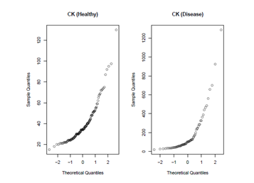
Figure 1 Q-Q plots of marker CK. Values from both the diseased and the healthy groups are not normally distributed, therefore, Box-Cox transformation is needed.
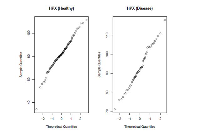
Figure 2 Q-Q plots of marker HPX. Values from both the diseased and the healthy groups are normally distributed.
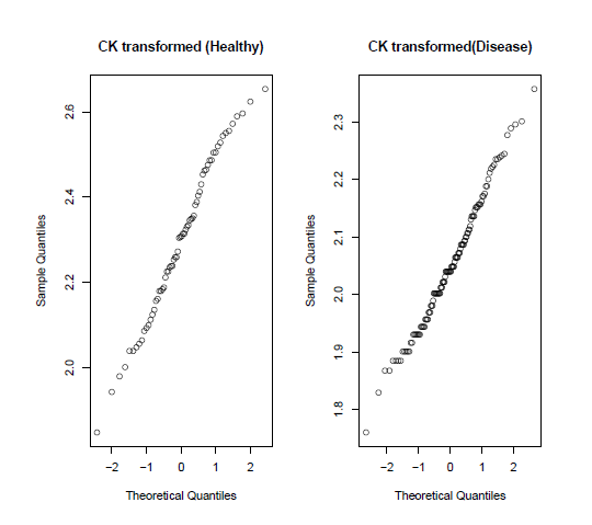
Figure 3 Q-Q plots of the Box-Cox transformed values of marker CK. After Box-Cox transformation, the values from both the diseased and the healthy groups are normally distributed.
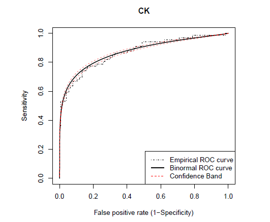
Figure 4 The estimated binormal ROC curve (bold), empirical ROC curve (step line) and the 95% confidence bands (CB) of the ROC curve. The binormal ROC curve and the corresponding Working Hotelling confidence band22 are fitted on the Box-Cox transformed values of marker CK.
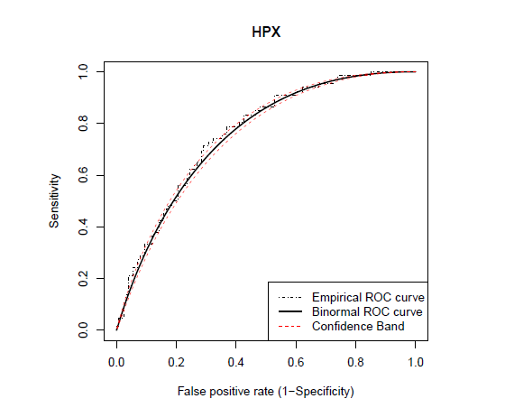
Figure 5 The estimated binormal ROC curve (bold), empirical ROC curve (step line) and the 95% confidence bands (CB) of the ROC curve. The binormal ROC curve and the corresponding Working Hotelling confidence band22 are fitted on the original values of marker HPX.

Table 2 gives the contingency table for marker CK at the cut-off point associated with the Youden index, which can be calculated from (4) using the binormal model. For table 3, the optimal cut-off point for the diagnosis based on marker CK is determined by maximizing the DOR or equivalently, the logarithm of DOR, i.e.,

c OR = max c { log( DOR( c ) )=log( Φ( μ 1 c σ 1 ) )+log( Φ( c μ 2 σ 2 ) )log( Φ( c μ 1 σ 1 ) )log( Φ( μ 2 c σ 2 ) ) } MathType@MTEF@5@5@+= feaagKart1ev2aaatCvAUfeBSjuyZL2yd9gzLbvyNv2CaerbuLwBLn hiov2DGi1BTfMBaeXatLxBI9gBaerbd9wDYLwzYbItLDharqqtubsr 4rNCHbGeaGqkY=xjYJH8sqFD0xXdHaVhbbf9v8qqaqFr0xc9pk0xbb a9q8WqFfeaY=biLkVcLq=JHqpepeea0=as0Fb9pgeaYRXxe9vr0=vr 0=vqpWqaaeaabiGaciaacaqabeaadaqaaqaaaOqaaKqzGeaeaaaaaa aaa8qacaWGJbGcdaWgaaqcbasaaKqzadGaam4taiaadkfaaSqabaqc LbsacqGH9aqpciGGTbGaaiyyaiaacIhakmaaBaaajeaibaqcLbmaca WGJbaaleqaaOWaaiWaaeaajugibiGacYgacaGGVbGaai4zaOWaaeWa aeaajugibiaadseacaWGpbGaamOuaOWaaeWaaeaajugibiaadogaaO GaayjkaiaawMcaaaGaayjkaiaawMcaaKqzGeGaeyypa0JaciiBaiaa c+gacaGGNbGcdaqadaqaaKqzGeGaeuOPdyKcdaqadaqaamaalaaaba qcLbsacqaH8oqBkmaaBaaajeaibaqcLbmacaaIXaaaleqaaKqzGeGa eyOeI0Iaam4yaaGcbaqcLbsacqaHdpWCkmaaBaaajeaibaqcLbmaca aIXaaaleqaaaaaaOGaayjkaiaawMcaaaGaayjkaiaawMcaaKqzGeGa ey4kaSIaciiBaiaac+gacaGGNbGcdaqadaqaaKqzGeGaeuOPdyKcda qadaqaamaalaaabaqcLbsacaWGJbGaeyOeI0IaeqiVd0McdaWgaaqc basaaKqzadGaaGOmaaWcbeaaaOqaaKqzGeGaeq4WdmNcdaWgaaqcba saaKqzadGaaGOmaaWcbeaaaaaakiaawIcacaGLPaaaaiaawIcacaGL PaaajugibiabgkHiTiGacYgacaGGVbGaai4zaOWaaeWaaeaajugibi abfA6agPWaaeWaaeaadaWcaaqaaKqzGeGaam4yaiabgkHiTiabeY7a TPWaaSbaaKqaGeaajugWaiaaigdaaSqabaaakeaajugibiabeo8aZP WaaSbaaKqaGeaajugWaiaaigdaaSqabaaaaaGccaGLOaGaayzkaaaa caGLOaGaayzkaaqcLbsacqGHsislciGGSbGaai4BaiaacEgakmaabm aabaqcLbsacqqHMoGrkmaabmaabaWaaSaaaeaajugibiabeY7aTPWa aSbaaKqaGeaajugWaiaaikdaaSqabaqcLbsacqGHsislcaWGJbaake aajugibiabeo8aZPWaaSbaaKqaGeaajugWaiaaikdaaSqabaaaaaGc caGLOaGaayzkaaaacaGLOaGaayzkaaaacaGL7bGaayzFaaaaaa@A4D1@ .

For this data set, the DOR does not reach its maximum within the observed range of cut-off point, so we select a point on the boundary. The maximum CK value of 2.6535 is chosen to be the optimal cut-off point. This situation is not rare, as Bohning et al.4 concluded that the DOR criteria for optimizing the cut-off point can “easily lead to cut-off point on the boundary of the parameter range".


Diseased

Healthy

Diagnostic

>2.1837

47

17

test result1

≤2.1837

19

110

Table 2 Contingency table of marker CK at the optimal cut-off point with the Youden index ( c j =2.1837 MathType@MTEF@5@5@+= feaagKart1ev2aaatCvAUfeBSjuyZL2yd9gzLbvyNv2CaerbuLwBLn hiov2DGi1BTfMBaeXatLxBI9gBaerbd9wDYLwzYbItLDharqqtubsr 4rNCHbGeaGqkY=xjYJH8sqFD0xXdHaVhbbf9v8qqaqFr0xc9pk0xbb a9q8WqFfeaY=biLkVcLq=JHqpepeea0=as0Fb9pgeaYRXxe9vr0=vr 0=vqpWqaaeaabiGaciaacaqabeaadaqaaqaaaOqaaKqzGeGaam4yaO WaaSbaaSqaaKqzadGaamOAaaWcbeaajugibiabg2da9iaaikdacaGG UaGaaGymaiaaiIdacaaIZaGaaG4naaaa@420D@ )

1, the diagnosis is based on the Box-Cox transformed marker value


Diseased

Healthy

Diagnostic

> 2.6535 2 MathType@MTEF@5@5@+= feaagKart1ev2aaatCvAUfeBSjuyZL2yd9gzLbvyNv2CaerbuLwBLn hiov2DGi1BTfMBaeXatLxBI9gBaerbd9wDYLwzYbItLDharqqtubsr 4rNCHbGeaGqkY=xjYJH8sqFD0xXdHaVhbbf9v8qqaqFr0xc9pk0xbb a9q8WqFfeaY=biLkVcLq=JHqpepeea0=as0Fb9pgeaYRXxe9vr0=vr 0=vqpWqaaeaabiGaciaacaqabeaadaqaaqaaaOqaaiabg6da+iaaik dacaGGUaGaaGOnaiaaiwdacaaIZaGaaGynamaaCaaaleqabaqcLbma caaIYaaaaaaa@3FC2@

0

0

test result1

≤2.6535

66

127

Table 3 Contingency table of marker CK at the optimal cut-off point with the maximum DOR ( c OR =2.6535) MathType@MTEF@5@5@+= feaagKart1ev2aaatCvAUfeBSjuyZL2yd9gzLbvyNv2CaerbuLwBLn hiov2DGi1BTfMBaeXatLxBI9gBaerbd9wDYLwzYbItLDharqqtubsr 4rNCHbGeaGqkY=xjYJH8sqFD0xXdHaVhbbf9v8qqaqFr0xc9pk0xbb a9q8WqFfeaY=biLkVcLq=JHqpepeea0=as0Fb9pgeaYRXxe9vr0=vr 0=vqpWqaaeaabiGaciaacaqabeaadaqaaqaaaOqaaKqzGeGaaiikai aadogakmaaBaaaleaajugWaiaad+eacaWGsbaaleqaaKqzGeGaeyyp a0JaaGOmaiaac6cacaaI2aGaaGynaiaaiodacaaI1aGaaiykaaaa@4422@

1, The diagnosis is based on the Box-Cox transformed marker value.
2, Since the DOR does not reach its maximum within the observed range of cut-off point (as shown in Figure 6), the maximum CK value (2.6535) is thus chosen to be the optimal cut-off point.

Table 4 summarizes the point and interval estimates for the AUC, the Youden index ( J ) MathType@MTEF@5@5@+= feaagKart1ev2aaatCvAUfeBSjuyZL2yd9gzLbvyNv2CaerbuLwBLn hiov2DGi1BTfMBaeXatLxBI9gBaerbd9wDYLwzYbItLDharqqtubsr 4rNCHbGeaGqkY=xjYJH8sqFD0xXdHaVhbbf9v8qqaqFr0xc9pk0xbb a9q8WqFfeaY=biLkVcLq=JHqpepeea0=as0Fb9pgeaYRXxe9vr0=vr 0=vqpWqaaeaabiGaciaacaqabeaadaqaaqaaaOqaamaabmaabaqcLb saqaaaaaaaaaWdbiaadQeaaOWdaiaawIcacaGLPaaaaaa@3B5A@ and the diagnostic odds ratios (DOR) at the optimal cut-off point corresponding to the maximum Youden index ( c J ) MathType@MTEF@5@5@+= feaagKart1ev2aaatCvAUfeBSjuyZL2yd9gzLbvyNv2CaerbuLwBLn hiov2DGi1BTfMBaeXatLxBI9gBaerbd9wDYLwzYbItLDharqqtubsr 4rNCHbGeaGqkY=xjYJH8sqFD0xXdHaVhbbf9v8qqaqFr0xc9pk0xbb a9q8WqFfeaY=biLkVcLq=JHqpepeea0=as0Fb9pgeaYRXxe9vr0=vr 0=vqpWqaaeaabiGaciaacaqabeaadaqaaqaaaOqaaabaaaaaaaaape WaaeWaaeaajugibiaadogakmaaBaaajeaibaqcLbmacaWGkbaaleqa aaGccaGLOaGaayzkaaaaaa@3DC1@  and the maximum DOR( c OR ) MathType@MTEF@5@5@+= feaagKart1ev2aaatCvAUfeBSjuyZL2yd9gzLbvyNv2CaerbuLwBLn hiov2DGi1BTfMBaeXatLxBI9gBaerbd9wDYLwzYbItLDharqqtubsr 4rNCHbGeaGqkY=xjYJH8sqFD0xXdHaVhbbf9v8qqaqFr0xc9pk0xbb a9q8WqFfeaY=biLkVcLq=JHqpepeea0=as0Fb9pgeaYRXxe9vr0=vr 0=vqpWqaaeaabiGaciaacaqabeaadaqaaqaaaOqaaKqzGeaeaaaaaa aaa8qacaWGebGaam4taiaadkfakmaabmaabaqcLbsacaWGJbqcfa4a aSbaaSqaaKqzadGaam4taiaadkfaaSqabaaakiaawIcacaGLPaaaaa a@420F@ for marker CK. When the cut-off point selected corresponds to the maximum DOR, the estimate for the DOR is infinity and therefore, no valid confidence interval can be calculated. Even at the optimal cut-off point with the Youden index, the DOR estimate still has a relatively wide confidence interval. However, both ROC indices, i.e., the AUC and the Youden index always yield bounded confidence intervals within the range of [0,1].


AUC

J

DOR( c J ) MathType@MTEF@5@5@+= feaagKart1ev2aaatCvAUfeBSjuyZL2yd9gzLbvyNv2CaerbuLwBLn hiov2DGi1BTfMBaeXatLxBI9gBaerbd9wDYLwzYbItLDharqqtubsr 4rNCHbGeaGqkY=xjYJH8sqFD0xXdHaVhbbf9v8qqaqFr0xc9pk0xbb a9q8WqFfeaY=biLkVcLq=JHqpepeea0=as0Fb9pgeaYRXxe9vr0=vr 0=vqpWqaaeaabiGaciaacaqabeaadaqaaqaaaOqaaKqzGeaeaaaaaa aaa8qacaWGebGaam4taiaadkfakmaabmaabaqcLbsacaWGJbqcfa4a aSbaaSqaaKqzadGaamOsaaWcbeaaaOGaayjkaiaawMcaaaaa@4133@

DOR( c OR ) MathType@MTEF@5@5@+= feaagKart1ev2aaatCvAUfeBSjuyZL2yd9gzLbvyNv2CaerbuLwBLn hiov2DGi1BTfMBaeXatLxBI9gBaerbd9wDYLwzYbItLDharqqtubsr 4rNCHbGeaGqkY=xjYJH8sqFD0xXdHaVhbbf9v8qqaqFr0xc9pk0xbb a9q8WqFfeaY=biLkVcLq=JHqpepeea0=as0Fb9pgeaYRXxe9vr0=vr 0=vqpWqaaeaabiGaciaacaqabeaadaqaaqaaaOqaaKqzGeaeaaaaaa aaa8qacaWGebGaam4taiaadkfakmaabmaabaqcLbsacaWGJbqcfa4a aSbaaSqaaKqzadGaam4taiaadkfaaSqabaaakiaawIcacaGLPaaaaa a@420F@

Point Est.

0.8721

0.6113

19.9650

inf

95% C.I.

(0.8157, 0.9284)

(0.5132, 0.7093)

(7.65 , 33.48)

-

Table 4 Summary of point and interval estimates about the AUC, the Youden index ( J ) MathType@MTEF@5@5@+= feaagKart1ev2aaatCvAUfeBSjuyZL2yd9gzLbvyNv2CaerbuLwBLn hiov2DGi1BTfMBaeXatLxBI9gBaerbd9wDYLwzYbItLDharqqtubsr 4rNCHbGeaGqkY=xjYJH8sqFD0xXdHaVhbbf9v8qqaqFr0xc9pk0xbb a9q8WqFfeaY=biLkVcLq=JHqpepeea0=as0Fb9pgeaYRXxe9vr0=vr 0=vqpWqaaeaabiGaciaacaqabeaadaqaaqaaaOqaamaabmaabaqcLb saqaaaaaaaaaWdbiaadQeaaOWdaiaawIcacaGLPaaaaaa@3B5A@ and the diagnostic odds ratios (DOR) at the optimal cut-off point corresponding to the maximum Youden index ( c J ) MathType@MTEF@5@5@+= feaagKart1ev2aaatCvAUfeBSjuyZL2yd9gzLbvyNv2CaerbuLwBLn hiov2DGi1BTfMBaeXatLxBI9gBaerbd9wDYLwzYbItLDharqqtubsr 4rNCHbGeaGqkY=xjYJH8sqFD0xXdHaVhbbf9v8qqaqFr0xc9pk0xbb a9q8WqFfeaY=biLkVcLq=JHqpepeea0=as0Fb9pgeaYRXxe9vr0=vr 0=vqpWqaaeaabiGaciaacaqabeaadaqaaqaaaOqaaabaaaaaaaaape WaaeWaaeaajugibiaadogakmaaBaaajeaibaqcLbmacaWGkbaaleqa aaGccaGLOaGaayzkaaaaaa@3DC1@ and the maximum DOR( c OR ) MathType@MTEF@5@5@+= feaagKart1ev2aaatCvAUfeBSjuyZL2yd9gzLbvyNv2CaerbuLwBLn hiov2DGi1BTfMBaeXatLxBI9gBaerbd9wDYLwzYbItLDharqqtubsr 4rNCHbGeaGqkY=xjYJH8sqFD0xXdHaVhbbf9v8qqaqFr0xc9pk0xbb a9q8WqFfeaY=biLkVcLq=JHqpepeea0=as0Fb9pgeaYRXxe9vr0=vr 0=vqpWqaaeaabiGaciaacaqabeaadaqaaqaaaOqaaKqzGeaeaaaaaa aaa8qacaWGebGaam4taiaadkfakmaabmaabaqcLbsacaWGJbqcfa4a aSbaaSqaaKqzadGaam4taiaadkfaaSqabaaakiaawIcacaGLPaaaaa a@420F@ for marker CK

1, The cut-off estimate is for the Box-Cox transformed CK values.

In Figure 7, the joint confidence region of the sensitivity and the specificity at the optimal cut-off point associated with the Youden index are plotted for marker HPX, along with the rectangular region formed by respective confidence intervals of the sensitivity and the specificity after the Bonferroni correction. The Bonferroni-corrected method is commonly used for adjusting multiple testing in practice due to its straightforward application. However, it is known to give conservative results. Similarly, Figure 8 gives the joint confidence region of the AUC and the Youden index for marker HPX along with the rectangular Bonferroni region. From Figure 8, since the correlation between the AUC and the Youden index is very high, the advantages of the joint confidence region are significant.
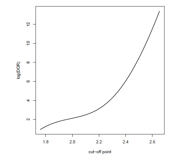
Figure 6 Logarithm of the DOR values across all possible values of the cut-off point for marker CK of the data set
Figure 7 The 95% joint confidence region of the sensitivity and the specificity at the optimal cut-off point associated with the Youden index for marker HPX. Since both the sensitivity and the specificity are given at the same cut-off point which is estimated by all samples from the two populations. Therefore, the sensitivity and the specificity at the optimal cut-off point are correlated (the sample correlation is −0.26 for this data set). Meanwhile, the rectangular region formed by respective individual confidence intervals adjusted by the Bonferroni correction is also plotted to compare with the joint elliptical region. The joint confidence region is estimated by the generalized inference approach, which automatically account for the correlation structure through simulations. The joint confidence region is given by the elliptical equation ( x0.7590 ) 2 0.1298 2 + ( y0.6179 ) 2 0.0956 2 =1 MathType@MTEF@5@5@+= feaagKart1ev2aaatCvAUfeBSjuyZL2yd9gzLbvyNv2CaerbuLwBLn hiov2DGi1BTfMBaeXatLxBI9gBaerbd9wDYLwzYbItLDharqqtubsr 4rNCHbGeaGqkY=xjYJH8sqFD0xXdHaVhbbf9v8qqaqFr0xc9pk0xbb a9q8WqFfeaY=biLkVcLq=JHqpepeea0=as0Fb9pgeaYRXxe9vr0=vr 0=vqpWqaaeaabiGaciaacaqabeaadaqaaqaaaOqaaabaaaaaaaaape WaaSaaaeaadaqadaqaaKqzGeGaamiEaiabgkHiTiaaicdacaGGUaGa aG4naiaaiwdacaaI5aGaaGimaaGccaGLOaGaayzkaaWaaWbaaSqabK qaGeaajugWaiaaikdaaaaakeaajugibiaaicdacaGGUaGaaGymaiaa ikdacaaI5aGaaGioaOWaaWbaaSqabKqaGeaajugWaiaaikdaaaaaaK qzGeGaey4kaSIcdaWcaaqaamaabmaabaqcLbsacaWG5bGaeyOeI0Ia aGimaiaac6cacaaI2aGaaGymaiaaiEdacaaI5aaakiaawIcacaGLPa aadaahaaWcbeqcbasaaKqzadGaaGOmaaaaaOqaaKqzGeGaaGimaiaa c6cacaaIWaGaaGyoaiaaiwdacaaI2aGcdaahaaWcbeqcbasaaKqzad GaaGOmaaaaaaqcLbsacqGH9aqpcaaIXaaaaa@604C@  with major axis being in the direction of vector ± ( 1,1.7237 ) T MathType@MTEF@5@5@+= feaagKart1ev2aaatCvAUfeBSjuyZL2yd9gzLbvyNv2CaerbuLwBLn hiov2DGi1BTfMBaeXatLxBI9gBaerbd9wDYLwzYbItLDharqqtubsr 4rNCHbGeaGqkY=xjYJH8sqFD0xXdHaVhbbf9v8qqaqFr0xc9pk0xbb a9q8WqFfeaY=biLkVcLq=JHqpepeea0=as0Fb9pgeaYRXxe9vr0=vr 0=vqpWqaaeaabiGaciaacaqabeaadaqaaqaaaOqaaKqzGeaeaaaaaa aaa8qacqGHXcqSkmaabmaabaqcLbsacaaIXaGaaiilaiabgkHiTiaa igdacaGGUaGaaG4naiaaikdacaaIZaGaaG4naaGccaGLOaGaayzkaa WaaWbaaSqabKqaGeaajugWaiaadsfaaaaaaa@4621@ and with point (0.7590,0.6179) as the origin. The individual confidence intervals are calculated by the lower and upper 0.05/4 percentiles of the simulated generalized pivotal quantities. The 97.5% adjusted confidence interval for sensitivity is (0.6418,0.8370), and that for specificity is (0.4957,0.7188).
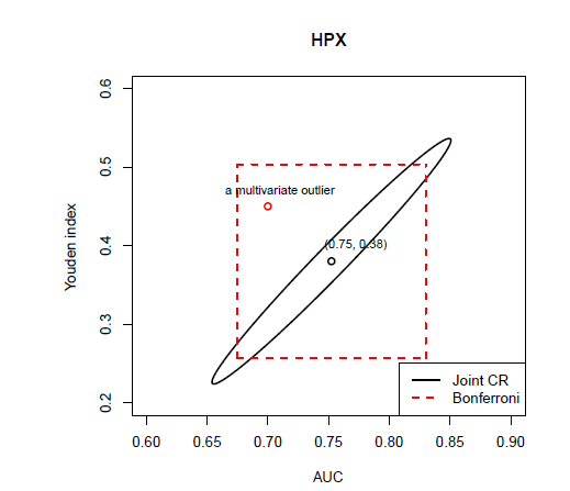
Figure 8 The 95% joint confidence region of the AUC and the Youden index and the rectangular region formed by respective individual confidence intervals adjusted by the Bonferroni correction for marker HPX. The joint confidence region is estimated by the large sample delta method, for which the variance matrix of AUC and Youden index is calculated analytically. The joint confidence region is given by the elliptical equation ( x0.7523 ) 2 0.1840 2 + ( y0.3802 ) 2 0.0146 2 =1 MathType@MTEF@5@5@+= feaagKart1ev2aaatCvAUfeBSjuyZL2yd9gzLbvyNv2CaerbuLwBLn hiov2DGi1BTfMBaeXatLxBI9gBaerbd9wDYLwzYbItLDharqqtubsr 4rNCHbGeaGqkY=xjYJH8sqFD0xXdHaVhbbf9v8qqaqFr0xc9pk0xbb a9q8WqFfeaY=biLkVcLq=JHqpepeea0=as0Fb9pgeaYRXxe9vr0=vr 0=vqpWqaaeaabiGaciaacaqabeaadaqaaqaaaOqaaabaaaaaaaaape WaaSaaaeaadaqadaqaaKqzGeGaamiEaiabgkHiTiaaicdacaGGUaGa aG4naiaaiwdacaaIYaGaaG4maaGccaGLOaGaayzkaaWaaWbaaSqabK qaGeaajugWaiaaikdaaaaakeaajugibiaaicdacaGGUaGaaGymaiaa iIdacaaI0aGaaGimaOWaaWbaaSqabKqaGeaajugWaiaaikdaaaaaaK qzGeGaey4kaSIcdaWcaaqaamaabmaabaqcLbsacaWG5bGaeyOeI0Ia aGimaiaac6cacaaIZaGaaGioaiaaicdacaaIYaaakiaawIcacaGLPa aadaahaaWcbeqcbasaaKqzadGaaGOmaaaaaOqaaKqzGeGaaGimaiaa c6cacaaIWaGaaGymaiaaisdacaaI2aGcdaahaaWcbeqcbasaaKqzad GaaGOmaaaaaaqcLbsacqGH9aqpcaaIXaaaaa@602E@  with major axis being in the direction of vector ± ( 1,1.5975 ) T MathType@MTEF@5@5@+= feaagKart1ev2aaatCvAUfeBSjuyZL2yd9gzLbvyNv2CaerbuLwBLn hiov2DGi1BTfMBaeXatLxBI9gBaerbd9wDYLwzYbItLDharqqtubsr 4rNCHbGeaGqkY=xjYJH8sqFD0xXdHaVhbbf9v8qqaqFr0xc9pk0xbb a9q8WqFfeaY=biLkVcLq=JHqpepeea0=as0Fb9pgeaYRXxe9vr0=vr 0=vqpWqaaeaabiGaciaacaqabeaadaqaaqaaaOqaaKqzGeaeaaaaaa aaa8qacqGHXcqSkmaabmaabaqcLbsacaaIXaGaaiilaiaaigdacaGG UaGaaGynaiaaiMdacaaI3aGaaGynaaGccaGLOaGaayzkaaWaaWbaaS qabKqaGeaajugWaiaadsfaaaaaaa@453B@ and with point (0.7523,0.3802) as the origin. The adjusted individual confidence intervals are calculated by the standard z-test at the confidence level of 97.5%, and it is (0.6747,0.8300) for the AUC and (0.2571,0.5033) for the Youden index. Since the AUC and Youden index are highly correlated, the rectangular region formed by Bonferroni approach is very conservative (as its area is much larger than that of the ellipse) and has less likelihood to successfully reject the multivariate outliers (e.g., point (0.7,0.45) in red).

Summary and discussion

Logistic regression and its corresponding odds ratio are the most popular measures of association between a continuous or categorical variable with a binary outcome in epidemiology, but it often produces results that are puzzling and misleading. A predictor with a large DOR does not necessarily yield a good prediction. Also, the DOR is not a proper measure of prediction accuracy for a strongly associated variable since the DOR will be very large and even close to infinity with wild confidence intervals. Henceforth, we need alternative approaches for evaluating strong association. In this paper, we recommend the use of the Receiver Operating Characteristic (ROC) curve. The most straightforward parametric approach to estimate the ROC curve and make inference about the ROC curve and its related summary indices is the binormal model.

The classical binormal model with two parameters has some limitations. Specifically, it does not fit well for “degenerate" data set. Metz and Pan40 suggested that the fitted ROC curve by the classical binormal model always lie partly below the diagonal line, and such phenomena is especially obvious for degenerate data. The sensitivity is not a monotonic increasing function with respect to the false positive rate, as is supposed to be by the ROC theory. Therefore, for such degenerate data, the binormal ROC curve is not “proper". Alternative parametric models were proposed when the conventional binormal model is no longer appropriate, including the “proper" binormal model41 and the “proper" bigamma model.41 Particularly, the “proper" binormal model contains three parameters by making diagnostic decisions based upon some monotonic transformations of the likelihood ratio of the bi-normally distributed random marker values. Unlike the two-parameter classical binormal model, the ROC-related indices may not have closed-form solutions expressed by the three parameters, which can be an interesting problem for future research.

When normality is not satisfied for either the diseased or the healthy population, it is a common practice to use Box-Cox transformation to achieve binormality in diagnostic studies. This is achieved due to the fact that ROC curve is invariant under monotonic transformations. An issue about the application of the binormal model in the ROC context is that it is not a very robust approach under violations of binormality assumption.42 Sometimes it is impossible to approximate normality well enough for both populations under a common transformation with the same λ. In such situation, the non-parametric bootstrap methods based on empirical estimates or kernel-smoothed estimates of the ROC curves or its summary indices has been shown to perform very well and are easily applied. For example, see Faraggi and Reiser35 and Fluss et al.25 for single indices, Yin and Tian13 and Bantis et al.32 for joint inference.

If multiple variables are believed to associate with the binary outcome of interest collectively but not individually, it is recommended to combine the variables to a composite score or function. In the context of the ROC analysis, researchers have proposed combining the multiple predictors by maximizing the ROC indices, such as the AUC or the Youden index.4347,11 After a composite score is obtained, the binormal model discussed here is readily applied for the composite score to make inference about the prediction accuracy when all variables are combined.

Acknowledgments

None.

Conflicts of interest

None.

References

  1. Kraemer HC. Reconsidering the odds ratio as a measure of 2x2 association in a population. Stat Med. 2004;23(2):257–270.
  2. Pepe MS, Janes H, Longton G, et al. Limitations of the odds ratio in gauging the performance of a diagnostic, prognostic, or screening marker. Am J Epidemiol. 2004;159(9):882–890.
  3. Glas AS, Lijmer JG, Prins MH, et al. The diagnostic odds ratio: a single indicator of test performance. J Clin Epidemiol. 2003; 56(11):1129–1135.
  4. Bohning D, Holling H, Patilea V. A limitation of the diagnostic-odds ratio in determining an optimal cut-off value for a continuous diagnostic test. Stat Methods Med Res. 2011;20(5):541–550.
  5. Shapiro DE. Zhou XH, McClish DK, et al. Statistical methods in diagnostic medicine, Wiley-Interscience; 2009:569.
  6. Zhou XH, McClish DK, Obuchowski NA. Statistical methods in diagnostic medicine, Wiley-Interscience; 2009:569.
  7. Pepe MS. The statistical evaluation of medical tests for classification and prediction.Oxford University Press, USA; 2004.
  8. Zou KH, Liu A, Bandos A, et al. Statistical evaluation of diagnostic performance: topics in ROC analysis. CRC Press, USA; 2010:245.
  9. Bamber D. The area above the ordinal dominance graph and the area below the receiver operating characteristic graph. Journal of Mathematical Psychology. 1975;12(4):387–415.
  10. Perkins NJ, Schisterman EF. The inconsistency of optimal cutpoints obtained using two criteria based on the receiver operating characteristic curve. Am J Epidemiol. 2006;163(7):670–675.
  11. Zou KH, Yu CR, Liu K, et al. Optimal thresholds by maximizing or minimizing various metrics via roc-type analysis. Academic radiology. 2013;20(7):807– 815.
  12. Schisterman EF, Perkins N. Confidence intervals for the youden index and corresponding optimal cut-point. Communications in Statistics Simulation and Computation R ⃝. 2007;36(3):549–563.
  13. Yin J, Tian L. Joint confidence region estimation for area under roc curve and youden index. Stat Med. 2014;33(6):985–1000.
  14. Gail MH, Green SB. A generalization of the one-sided two-sample kolmogorov-smirnov statistic for evaluating diagnostic tests. Biometrics. 1976;32(3):561–570.
  15. Rucker G, Schumacher M. Summary roc curve based on a weighted youden index for selecting an optimal cutpoint in meta- analysis of diagnostic accuracy. Stat Med. 2010;29(30):3069–3078.
  16. Dorfman DD, Alf E. Maximum-likelihood estimation of parameters of signal-detection theory and determination of confidence intervals? rating-method data. Journal of mathematical psychology. 1969;6(3):487–496.
  17. Hanley JA. The robustness of the “binormal” assumptions used in fitting roc curves. Medical Decision Making. 1988;8(3):197–203.
  18. Zou KH, Hall W. Two transformation models for estimating an roc curve derived from continuous data. Journal of Applied Statistics. 2000;27(5):621–631.
  19. Hanley JA. The robustness of the” binormal” assumptions used in fitting roc curves. Med Decis Making. 1988;8(3):197–203.
  20. Linnet K. Comparison of quantitative diagnostic tests: type i error, power, and sample size. Stat Med. 1987;6(2):147–158.
  21. Ma G, Hall W. Confidence bands for receiver operating characteristic curves. Med Decis Making. 1933;13(3):191–197.
  22. Working H, Hotelling H. Applications of the theory of error to the interpretation of trends. Journal of the American Statistical Association. 1929;24(165A):73–85.
  23. Demidenko E. Confidence intervals and bands for the binormal roc curve revisited. J Appl Stat. 2012;39(1):67–79.
  24. Yin J, Tian L. Generalized inference confidence band for binormal roc curve. Statistics in Biopharmaceutical Research (just-accepted). 2015:1–34.
  25. Fluss R, Faraggi D, Reiser B (2005) Estimation of the youden index and its associated cutoff point. Biom J 47(4): 458-472.
  26. Lai CY, Tian L, Schisterman EF. Exact confidence interval estimation for the youden index and its corresponding optimal cut-point. Comput Stat Data Anal. 2012;56(5):1103–1114.
  27. Wieand S, Gail MH, James BR, et al. A family of nonparametric statistics for comparing diagnostic markers with paired or unpaired data. Biometrika. 1989;76(3):585–592.
  28. Molodianovitch K, Faraggi D, Reiser B. Comparing the areas under two correlated roc curves: Parametric and non-parametric approaches. Biom J. 2006;48(5):745-757.
  29. Tian L. Confidence intervals for p(y1 >y2) with normal outcomes in linear models. Stat Med. 2008;27(21):4221–4237.
  30. Li CR, Liao CT, Liu JP. On the exact interval estimation for the difference in paired areas under the roc curves. Stat Med. 2008; 27(2):224–242.
  31. Yin J, Tian L. Joint inference about sensitivity and specificity at the optimal cut-off point associated with youden index. Computational Statistics & Data Analysis. 2014;77:1–13.
  32. Bantis LE, Nakas CT, Reiser B. Construction of confidence regions in the roc space after the estimation of the optimal youden index-based cut-off point. Biometrics. 2014;70(1):212–223.
  33. Tsui KW, Weerahandi S. Generalized p-values in significance testing of hypotheses in the presence of nuisance parameters. Journal of the American Statistical Association. 1989;84(406):602–607.
  34. Weerahandi S. Generalized confidence intervals. J Am Stat Assoc. 1993;88(423):899–905.
  35. Faraggi D, Reiser B. Estimation of the area under the roc curve. Stat Med. 2002;21(20):3093–3106.
  36. Schisterman EF, Faraggi D, Reiser B, et al. Roc analysis for markers with mass at zero. Statistics in medicine. 2006;25(4):623–638.
  37. Schisterman EF, Reiser B, Faraggi D. Roc analysis for markers with mass at zero. Statistics in medicine. 2006;25(4):623–638.
  38. Sakia R. The box-cox transformation technique: a review. The statistician. 1992;169–178.
  39. Percy ME, Andrews DF, Thompson MW. Duchenne muscular dystrophy carrier detection using logistic discrimination: serum creatine kinase, hemopexin, pyruvate kinase, and lactate dehydrogenase in combination. American journal of medical genetics.1982;13(1): 27–38.
  40. Metz CE, Pan X. Proper binormal roc curves: theory and maximum-likelihood estimation. J Math Psychol. 1999;43(1):1–33.
  41. Dorfman DD, Berbaum KS, Metz CE, et al. Proper receiver operating characteristic analysis: the bigamma model. Acad Radiol. 1997;4(2):138–149.
  42. WALSH SJ. Limitations to the robustness of binormal roc curves: effects of model misspecification and location of decision thresholds on bias, precision, size and power. Stat Med. 1997;16(6):669–679.
  43. Kang L, Liu A, Tian L. Linear combination methods to improve diagnostic/prognostic accuracy on future observations. Stat Methods Med Res. 2013;22(4):1359–1380.
  44. Liu C, Liu A, Halabi S. A min-max combination of biomarkers to improve diagnostic accuracy. Stat Med. 2011;30(16):2005–2014.
  45. Pepe MS, Thompson ML. Combining diagnostic test results to increase accuracy. Biostatistics. 2000;1(2):123–140.
  46. Su JQ, Liu JS. Linear combinations of multiple diagnostic markers. J Am Stat Assoc. 1993;88(424):1350–1355.
  47. Yin J, Tian L. Optimal linear combinations of multiple diagnostic biomarkers based on youden index. Stat Med. 2014;33(8):14.
Creative Commons Attribution License

©2017 Yin, et al. This is an open access article distributed under the terms of the, which permits unrestricted use, distribution, and build upon your work non-commercially.