Confidence intervals for the risk ratio when analyzing bioassays in the presence of over dispersion

doi:10.15406/bbij.2015.02.00050

eISSN: 2378-315X

Biometrics & Biostatistics International Journal

Research Article Volume 2 Issue 7

Confidence intervals for the risk ratio when analyzing bioassays in the presence of over dispersion

Frank Schaarschmidt

Verify Captcha

Regret for the inconvenience: we are taking measures to prevent fraudulent form submissions by extractors and page crawlers. Please type the correct Captcha word to see email ID.

Leibniz Universität Hannover, Germany

Correspondence: Frank Schaarschmidt, Institute of Biostatistics, Leibniz Universit, Tel 49 511 762 5821, Fax 49 511 762 4966

Received: August 07, 2015 | Published: October 26, 2015

Citation: Schaarschmidt F. Confidence intervals for the risk ratio when analyzing bioassays in the presence of over dispersion. Biom Biostat Int J. 2015;2(7):200-208. DOI: 10.15406/bbij.2015.02.00050

Download PDF

Abstract

Many bioassays that assess toxicity or mutagenicity give rise to clustered binomial data with relatively few replicated experimental units per treatment group. Confidence intervals for the risk ratio to control can then be used to interpret the relevance of effect size or test hypotheses of superiority, non-inferiority or equivalence. A frequently observed property of clustered binomial data is overdispersion. So far, the available large-sample confidence interval methods for ratios of proportions in presence of overdispersion have been validated for use in epidemiological settings with high numbers of clusters per exposure group.

In this paper, the coverage probability and symmetry of non-coverage of several available methods is investigated in an extensive Monte-Carlo simulation study, for the small number of replications that are typical for a number of bioassays. An additional method is proposed that combines profile deviance intervals with the method of variance recovery. So far available confidence intervals have far too low coverage probabilities in the simulated settings. Their performance can be improved by restricting estimators of dispersion not to fall below the binomial variance and by using pooled dispersion estimators. The newly proposed method outperforms the so far available methods by showing coverage probabilities closest to the nominal level. All discussed methods are made available in an add-on package for the R software.

Keywords: ratio of proportions, extra-binomial variance, beta-binomial, monte carlo simulation, coverage probability, bioassay, small sample performance

Abbreviations

FN, fieller-type intervals applied on the observed proportions; BM, binomial MOVER-R-Wilson method after summing-up observed counts across replications; LOD, asymptotic method on the log-scale; accounting for overdispersion via residual variation; FOD, fieller-bailey-type interval accounting for over dispersion via residual variance; LBB, delta method on the log-scale under the beta-binomial assumption; FBB, fieller-bailey-type interval under beta-binomial assumption; QBM, MOVER-R for quasibinomial profile deviance intervals

Introduction

Various bioassays give rise to replicated binomial count data. For example, in ecotoxicological assays, fish larvae or daphnids in several tanks are exposed to different dosages of a substance and the number of dead or immobile animals per tank is used to assess the hazardousness of the substance. Usually, a small number of replicated tanks are used for each dosage under consideration. If some experimental conditions differ between tanks such that the proportion of dead or immobile daphnids is effected, counted numbers may show higher variance than expected under the binomial assumption, i.e., extra-binomial variability or overdispersion. Similar situations arise in the in-vivo micronucleus assay: the number of cells showing micronuclei is counted for a given number of exposed cells for each (randomized) animal, with the aim to assess the substances' potential to cause cytogenetic damage. Also here, a limited number of replications per dosage is performed, such that differences between animals in the in-vivo micronucleus animals may cause overdispersion. In summary, bioassays that lead to binomial data, often contain clustered replication, and thus make it possible to account for overdispersion in the data. However, the number of replications or clusters per treatment group that allows to assess the extend of overdispersion, is rather limited.

In the statistical analysis of such bioassays, major interest is usually in comparisons to the untreated control group. While a test on significance for the overall effect of dosage of the substance may be of preliminary interest, usually more detailed interpretation for the single dosages is required: Confidence intervals for the effect of given dosages compared to the untreated control or a positive control are required to interpret the toxicological relevance of the observed effect size. Tests of non-inferiority (or equivalence) for given dosages compared to an untreated control¹ may be more important than an overall test on significant change in the event rates: In toxicological assessment, confidence is needed primarily when claiming no effect. Both approaches require an interpretable definition of the change of the rate of the detrimental event (death or immobility, presence of micronculei, malformations, etc.) compared to the control treatment: for judging relevance of an effect size or for the definition of a particular non-inferiority margin.¹

For this reason, this paper is focused on the ratio of proportions (risk ratio). Compared to the plenty of publications considering the construction of confidence intervals for a single binomial proportion, as well as for differences, ratios or odds-ratios of binomial proportions, the construction confidence intervals for risk ratios of overdispersed binomial data has received only little attention.^2,3 The available methods are all asymptotic methods. Their construction and their evaluation is usually motivated by their application to epidemiological studies, where the absence or presence of a disease is counted for a given number of individuals in clusters. In this context, clustering of individuals may arise from humans being clustered in families or locations or from repeated measurements within a given animal, or repeated animals within a given farm when veterinary epidemiology is concerned. In these settings, there is usually a relatively large number of clusters available (many families or locations, many farms or animals), such that simple asymptotic methods work well and the estimation of the overdispersion parameters is rather precise. This is not the case in bioassays that are the focus of this paper. In epidemiological settings it is also rather improbable to observe no single disease case across all clusters in one of the groups to be compared, or, conversely, to observe only disease cases across all clusters in one group. Such outcomes, however, plausibly occur in the untreated control groups of bioassays and may cause problems with Wald-type test and related confidence intervals.⁴ Finally, in epidemiological studies, major interest is usually in estimation, such that the statistical evaluation of confidence interval methods for the risk ratio does plausibly focus on (two-sided) coverage probability and interval width. In the case of bioassays, estimation as well as related hypothesis tests are of interest. In testing, one-sided hypotheses are most relevant and may involve margins of non-inferiority.

In consequence, previous recommendations of confidence intervals methods for risk ratios of overdispersed data, motivated by epidemiological applications, cannot directly transferred to their application to bioassays. In this paper, previously proposed confidence intervals are thus investigated with special focus on small to very small number of clusters (i.e. replications) and the possibility that all observations in one group may show the same event. Due to the need of estimation as well as one-sided non-inferiority tests, two-sided as well as one-sided coverage probabilities are investigated for a wide range of parameter combinations. Further, a new method based on a straightforward combination of profile deviance intervals, e.g,^5,6 and the method of variance recovery⁷ is proposed and is shown to clearly outperform existing approaches under the assumption of a common level of overdispersion.

Material and methods

Parameter and hypotheses of interest

Assume an experimental setup, where for each treatment i, there are Ji replicated experimental units (tanks, cages, animals, petri dishes, etc.) with index j = 1, …, Ji. In each experimental unit there is a number of nij biological units under observation, and the number of events of interest, xij, is counted in unit ij. These counted events may be death (or survival) of animals, mobility (or immobility) of daphnids, presence or absence of micronuclei, etc. Consider the comparison of one dose group, i = 1, to the untreated control, i = 0. Denote the unknown probability of events in the two groups by i, and parameter of interest is the risk ratio $p = \frac{π_{1}}{π_{0}}$ . Beside estimating ρ and displaying the uncertainty of this estimate in terms of a 95% confidence interval, decisions concerning one-sided hypotheses on tests on non-inferiority or superiority may be of interest. The particular choice of non-inferiority margins, ρ0, may be fixed by convention, compare¹ suggesting ρ0 = 0.75 or ρ0 = 0.8 for certain applications. In other situations, it might be a matter of debate. Although general focus is in valid two-sided confidence intervals (i.e., with coverage probability close to the nominal level), it will be further investigated whether confidence intervals do also provide valid upper and lower confidence limits and can thus be used to perform (approximate) level α test for one-sided hypotheses.

Overdispersed binomial data

There are two well-known approaches to model overdispersion in binomial data.⁸ The quasibinomial approach models overdispersion by assuming the variance-mean-dependency
$V^{Q B} (X_{i j}) = ϕ n_{i j} π_{i j} (1 - π_{i j})$ ,
where ϕ is the overdispersion parameter that inflates the binomial variance term by a common fold, independent of the sample size nij. In this parameterization, the binomial assumption,
$V^{B} (X_{i j}) = n_{i j} π_{i j} (1 - π_{i j})$ , is met for ϕ = 1.

The beta-binomial distribution derives from a beta mixture of binomial distributions, i.e.,
$π_{i j} \sim B e t a (a_{1}, b_{1})$ , and $x_{i j} \sim B i n o m i a l (n_{i j}, π_{i j})$ (1)

where $E (π_{i j}) = \frac{a_{i}}{(a_{i} + b_{i})}$ , $E (x_{i j}) = \frac{n_{i i} a_{i}}{(a_{i} + b_{i})}$ [9]. Denote the sum of the two parameters of the beta-parameters by $a_{i}^{*} = a_{i} + b_{i}$ . The variance of beta-binomial counts, $v^{B B} (X_{i j})$ is a function of nij, πij, $a_{i}^{*}$ [5,9]. When $a_{i}^{*}$ approaches $\infty$ , the variance of the beta-binomial counts approaches that of binomial counts. Here, the overdispersion relative to the binomial variance, $v^{B B} (X_{i j})$ , is denoted by $ϕ^{B B} = \frac{V^{B B} (X_{i j})}{V^{B} (X_{i j})}$ and is a function of nij and $a_{i}^{*}$ . This allows to choose $a_{i}^{*}$ given nij such that the over dispersion $a_{i}^{*}$ is a constant factor, namely $φ^{B B}$ .

Main interest here is in the performance of confidence interval methods in highly controlled laboratory settings. Under such conditions it can be assumed that nij is equal for all experimental units, ij. Under such conditions, the quasibinomial assumption on the variance mean dependency coincides with the variance-mean-dependency under the beta-binomial distribution.^5,9 Hence, methods are considered that are explicitly constructed for the beta-binomial distribution, as well as methods that account for overdispersion under the quasibinomial assumption.

Confidence interval methods

Fieller-type intervals applied on the observed proportions (FN):

Naively, the t-test for ratios, with a common variance estimator and the assumption of normal distributed residuals, may be used to test the above hypotheses, treating the observed proportions as the variable of interest, $y_{i j} = {\overset{⌢}{π}}_{i j}$ . The corresponding Fieller-type confidence interval can be obtained by analytically inverting the t-test statistic for ratios.¹⁰ The method assumes normal distribution and variance homogeneity for the observed proportions, which is clearly not the case in this application. This interval is referred to as FN.

Binomial MOVER-R-Wilson method after summing-up observed counts across replications (BM): It may be tempting to sum up the counts over experimental units within each treatment group, $x_{i} = \sum_{j = 1}^{j_{i}} x_{i j}, n_{i} = \sum_{j = 1}^{j_{i}} n_{i j}$ and apply a confidence interval for risk ratios under the assumption of binomial distribution, i.e., ignoring possible extra-binomial variation. As a place holder for the many available options, here the MOVER-R method proposed by² is used; this is computationally simple and was among the best methods in a recent comparative study under the binomial assumption by.¹¹ It is referred to as BM.

The two above methods are merely included here to illustrate the effects of either ignoring the mean-variance-relation and skewness implied by binomial distribution (FN) or the effect of applying binomial methods (BM) when data are indeed overdispersed binomial.

Asymptotic method on the log-scale, accounting for overdispersion via residual variation (LOD): Among other methods,³ investigate and recommend a method based on the delta method applied for the log risk ratios (called MR1 therein). It can be computed from:

$n_{i} = \sum_{j = 1}^{j_{i}} n_{i j}, x_{i} . = \sum_{j = 1}^{j_{i}} x_{i j,} {\hat{π}}_{i} = \frac{x_{i .} + 0.5}{n_{i .} + 1}, \hat{p} = \frac{{\hat{π}}_{1}}{{\hat{π}}_{0}}$ , ${\hat{u}}_{i} = (\frac{j_{i}}{j_{i} - 1}) \sum_{j = 1}^{j_{i}} \frac{{(x_{i j} - {\hat{π}}_{i .} n_{i j})}^{2}}{n_{i}^{2}}$ (2)

Where the variance is estimated from the residuals on the scale of the original observations. The interval is then given by:

$\hat{p} \exp (\pm z_{1 - \frac{α}{2}} \sqrt{\sum_{i = 0}^{1} \frac{{\hat{u}}_{1}}{{\hat{π}}_{i}^{2}}})$ (3)

By plugging-in the observed residual variance per treatment group i, this method does not assume a particular mean-variance relation and accounts for overdispersion in a more general way. However, if the number of replications per treatment, Ji, is small, these variance estimates might be unstable. Zaihra and Paul³ additionally consider a closely related method with a sandwich-type variance estimator, which performs worse in their simulation study, and is thus ignored here.

Fieller-Bailey-type interval accounting for overdispersion via residual variance (FOD): Using the estimators above,³ follow the approach of¹⁰ and¹² that accounts for the skewed distribution of the original Fieller statistic

$z = \frac{{\hat{π}}_{1} - p {\hat{π}}_{0}}{\sqrt{{\hat{v}}_{1} + p^{2} {\hat{v}}_{0}}}$

By considering the solutions of a cubic equation, with
$A = {\hat{π}}_{0}^{\frac{2}{3}} - z_{\frac{α}{2}}^{2} \frac{{\hat{v}}_{0}}{9 {\hat{π}}_{0}^{\frac{4}{3}}}, B = {({\hat{π}}_{1} {\hat{π}}_{0})}^{\frac{1}{3}}, C = {\hat{π}}_{1}^{\frac{2}{3}} - z_{\frac{α}{2}}^{2} \frac{{\hat{v}}_{1}}{9 {\hat{π}}_{1}^{\frac{4}{3}}}$

The interval (referred to as MR4 by³) can then be computed by

$[\max ((\frac{B - \sqrt{B^{2} - A C}}{A}), 0); {(\frac{B - \sqrt{B^{2} - A C}}{A})}^{3}]$

If A > 0 and B2 - AC > 0. If these two restrictions are not met, the interval has unbounded or disjoint solutions which do not provide meaningful interpretations of ρ. In the simulation study below, the interval $[0, \infty]$ is returned in such cases [3]. Again consider a closely related method that uses sandwich estimator for the variance of ${\hat{π}}_{i}$ instead. It is not considered here.

Delta method on the log-scale under the beta-binomial assumption (LBB): Lui et al.² propose methods that are constructed under the assumption of the beta-binomial distribution. Theoretically, the variance of ${\hat{π}}_{i}$ under this assumption is ${\hat{π}}_{i} (1 - π_{i}) ϕ^{B B} (n_{i, C_{i}}) / n_{i}$ where $ϕ^{B B} (n_{i, C_{i}})$ is the beta-binomial overdispersion factor, expressed as a function of the number under risk in each replication ij of treatment i, $ϕ^{B B} (n_{i, C_{i}})$ and of ci, the intraclass correlation coefficient. Under beta-binomial sampling, the intraclass correlation depends on $a_{i}^{*}$ via $c_{i} = 1 / (a_{1}^{*} + 1)$ .²

Lui et al.² estimate the intraclass correlation using

${\hat{c}}_{i} = \frac{B M S_{i} - W M S_{i}}{B M S_{i} + (n_{1}^{*} - 1) W M S_{i}}, w i t h - n_{1}^{*} = \frac{n_{i .}^{2} - n_{i j}^{2}}{(J_{i} - 1) n_{i}}$

Based on the between and within mean squared error of the observations,

$B M S_{i} = \frac{\sum_{j = 1}^{J_{1}} \frac{x_{i j}^{2}}{n_{i j}} - \frac{x_{i .}^{2}}{n_{i .}}}{J_{i} - 1}$ and $W M S_{i} = \frac{x_{i .} - \sum_{j = 1}^{J_{i}} \frac{x_{i j}^{2}}{n_{i j}}}{\sum_{j = 1}^{J_{1}} (n_{i j} - 1)}$

This leads to estimators for the beta-binomial overdispersion factor, and the related variance of the proportion estimator under the beta-binomial assumption, for each treatment group i separately:²

${\hat{ϕ}}^{B B} (n_{i}, {\hat{c}}_{i}) = \sum_{j = 1}^{J_{i}} n_{i j} (1 + (n_{i j} - 1) {\hat{c}}_{i}) / n_{i .}$ (5)

${\hat{v}}_{i}^{B B} = \frac{(1 - {\hat{π}}_{i}) {\hat{ϕ}}^{B}^{B} (n_{i_{1}} {\hat{c}}_{i})}{n_{i} {\hat{π}}_{i}}$ (6)

The asymptotic interval relying on the delta method applied for the log risk ratio [2] can be constructed by:
$\hat{p} \exp (\pm Z_{1} - α / 2 \sqrt{\sum_{i = 0}^{1} {\hat{v}}_{i}^{B B}})$ (7)

Fieller-Bailey-type interval under beta-binomial assumption: FBB: Lui et al.² consider a Fieller-type interval and its modification according to¹² under the beta-binomial distribution:
$A = {\hat{π}}_{0}^{2 / 3} - z_{α / 2}^{2} (1 - {\hat{π}}_{0}) ϕ^{B B} (n_{0}, {\hat{c}}_{0}) / (9 n_{0.} {\hat{π}}_{0}^{1 / 3}), B = {({\hat{π}}_{1} {\hat{π}}_{0})}^{1 / 3}$ and
$C = {\hat{π}}_{1}^{2 / 3} - z_{α / 2}^{2} (1 - {\hat{π}}_{1}) ϕ^{B B} (n_{1}, {\hat{c}}_{1}) / (9 n_{1.} {\hat{π}}_{1}^{1 / 3})$

As in Eq. (4), a meaningful interval can be calculated if A > 0 and B2 - AC > 0:

$[\max ({(\frac{B - \sqrt{B^{2} - A C}}{A})}^{3}, 0); {(\frac{B - \sqrt{B^{2} - A C}}{A})}^{3}]$ (8)

In the simulation study below, the interval $[0, \infty]$ is returned if A > 0 and B2-AC > 0. Following [2], in case of the extreme events ${\hat{π}}_{i} = 0$ or ${\hat{π}}_{i} = 1$ , is replaced by ${\hat{π}}_{i} = \frac{x_{i .} + 0.5}{n_{i} + 1}$ in the LBB and FBB method and their subsequent modifications.

Modifications of LOD, FOD, LBB, FBB by pooling and restricting the variance estimates: Lui et al² state, based on theoretical considerations and in the context of estimation problems that the intraclass correlation ci and the overdispersion $ϕ_{B B} (n_{i}, c_{i})$ cannot fall below 0 and 1, respectively. However, their estimates may fall below the boundaries imposed by the binomial assumption. For example, the event $x_{i 1} = x_{i 2} = .... = x_{i} j_{i}$ may lead to the unreasonable estimates $c_{i} < 0$ and $ϕ_{B B} (n_{i}, c_{i}) = 0$ . Moreover, interest here is in small sample laboratory experiments and estimating ci and $ϕ_{B B} (n_{i}, c_{i})$ separately for each treatment from very few replications Ji may result in over fitting. Then, the assumption of a common beta-binomial overdispersion parameter $ϕ_{^{B B}} (n_{i}, {\hat{c}}_{i})$ may lead to a more stable estimation with small sample sizes. Therefore, the methods LBB and FBB as well as LOD an FOD are simulated with the following additional restrictions and pooling of variance estimates:

LBB1, FBB1 refer to methods LBB, FBB with the beta-binomial overdispersion factor restricted to be at least 1, i.e., using $m a x (1, ϕ_{^{B B}} (n_{i}, {\hat{c}}_{i}))$ instead of $ϕ_{^{_{_{B B}}}} (n_{i}, {\hat{c}}_{i})$ in the equations (5,6)ff.
LBBp, FBBp refer to methods LBB, FBB with the intraclass correlation estimator using pooled observations across the groups, ${\hat{C}}_{.} = \frac{\sum_{i = 1}^{2} c_{i} n_{i}}{\sum_{i = 1}^{2} n_{i}}$ and $ϕ^{B B} (n_{i}, \hat{c} .)$ , instead of $ϕ^{B B} (n_{i}, \hat{c} .)$ in equations (5, 6)ff.
LBB1p, FBB1p combine the two approaches by using the group wise variance estimators with the pooled intraclass correlation estimator and restriction of the over dispersion parameter to be $\geq 1$ , that is, using $m a x (1, ϕ^{B B} (n_{i}, {\hat{c}}_{i}))$ instead of $ϕ^{B B} (n_{i}, \hat{c} .)$ in equations (5,6)ff. This procedure has been already suggested in the example evaluation of.²
LOD1, FOD1: refer to methods LOD, FOD, but the group wise variance estimators are restricted to be greater than or equal to the binomial variance estimate: using ${\hat{v}}_{i} = \max (\frac{{\hat{π}}_{i} (1 - {\hat{π}}_{i})}{n_{i .}}, (\frac{J_{i}}{J_{i} - 1}) \sum_{j = 1}^{J_{i}} \frac{{(x_{i j} - {\hat{π}}_{i .} n_{i j})}^{2}}{n_{i}^{2}})$ in Eq.(2)

MOVER-R for quasibinomial profile deviance intervals (QBM): An alternative option to obtain intervals for the risk ratio would be to fit a generalized linear model (GLM) under the quasibinomial assumption $V_{Q B} (X_{i j}) = ϕ n_{i j} π_{i j} (1 - π_{i j})$ , using a log-link, $n_{i j} = \log (π_{i j}), n_{i j} = β_{i}$ . Then the risk ratio can be estimated via $\exp (β_{1} - β_{0})$ and intervals for the difference $(β_{1} - β_{0})$ can be computed by the signed root profile deviance method.^6,5 However, with the current user-level implementations in R, fitting this model (glm, stats) and obtaining profile-deviance intervals (profile, confint, package MASS) suffers from numerical difficulties if at least one of the groups shows estimated success probabilities close or equal to 1 or equal to 0.

As a numerically stable work-around, the QBM method is proposed: A GLM with the quasibinomial assumption and logit link is fitted $n_{i j} = \log (π_{i j} / (1 - π_{i j})) = β_{i}$ . If the estimated dispersion parameter in the model fit falls below $1, {\hat{ϕ}}^{(Q B)} < 1$ , a binomial model is used instead (i.e., assuming $ϕ = 1$ ). For the βi, (1-α)--signed root profile deviance intervals can be computed, with limits denoted $[l_{\hat{β} 0}, u_{\hat{β} 0}], [l_{\hat{β} 1}, u_{\hat{β} 1}]$ and estimates denoted ${\hat{β}}_{i}$ . In R, these computations can be done in several packages, e.g. package MASS,⁵ or the add-on package mcprofile.¹³ Again, in extreme cases, the automatic search of values for the grid of parameter values for the deviance profile may fail in both packages. The signed root deviance is then computed over a pre-specified grid of parameter values,

$β_{i}^{*} = (- 10, - 9.5, ..., - 5, - 4.8, - 4.6, ...., 4.8, 5, 5.5, ...., 10)$

with elements $β_{i k}^{*}$ , k = 1,…, K. For each i and each k,

$t_{i k} = s i g n (β_{i k}^{*} - {\hat{β}}_{i}) \sqrt{\frac{d (β_{i k}^{*}, {\hat{β}}_{i'}) - d (β_{i}^{*}, {\hat{β}}_{i'})}{\hat{ϕ}}}$

is computed, where $s i g n (β_{i k}^{*} - {\hat{β}}_{i})$ retains the sign of the difference $β_{i k}^{*} - {\hat{β}}_{i}$ , $d (β_{i k}^{*} - {\hat{β}}_{i})$ is the deviance when replacing ${\hat{β}}_{i}$ by $β_{i k}^{*}$ while leaving all other parameters at their ML estimates, ${\hat{β}}_{i'}$ , $d (β_{i k}^{*} - {\hat{β}}_{i})$ is the deviance at the ML estimates, and $\hat{ϕ}$ is the dispersion estimate with all parameters at their ML estimates. For each parameter i, a cubic spline is fitted for tik depending on $β_{i k}^{*}$ and the cut points of the spline with quantiles of the t-distribution, $t_{α / 2, d f = d f r,} t_{1 - α / 2, d f = d f r}, d f r = \sum_{i = 1}^{I} (J_{i} - 1)$ is determined by linear interpolation between fitted values. When the binomial model is used, tik is replaced by

$Z_{i k} = s i g n ((β_{i k}^{*} - {\hat{β}}_{i})) \sqrt{d (β_{i k}^{*}, {\hat{β}}_{i'}) - d (β_{i}^{*}, {\hat{β}}_{i'})}$

And the quantiles of the standard normal distribution $Z_{α / 2}, Z_{1 - α / 2}$ , are used instead.

The interval bounds and ML estimates are transformed to the proportion scale using the inverse link, $[l_{i} - u_{i}] = [\frac{\exp (l_{\hat{β} i})}{1 + \exp (l_{\hat{β} i})}, \frac{\exp (u_{\hat{β} i})}{1 + \exp (u_{\hat{β} i})}], {\hat{π}}_{i} = \exp ({\hat{β}}_{i}) / (1 + \exp ({\hat{β}}_{i}))$ . These estimators and confidence limits are then used to compute intervals for ρ by the MOVER-R method.⁷ Eq. (9) of⁷ is recalled in the following as:

$[\frac{{\hat{π}}_{1} {\hat{π}}_{0} - \sqrt{{({\hat{π}}_{1} {\hat{π}}_{0})}^{2} - l_{1} u_{0} (2 \hat{π} - l_{1})} (2 {\hat{π}}_{0} - u_{0})}{u_{0} (2 {\hat{π}}_{0} - u_{0})}; \frac{{\hat{π}}_{1} {\hat{π}}_{0} - \sqrt{{({\hat{π}}_{1} {\hat{π}}_{0})}^{2} - u_{1} l_{0} (2 \hat{π} - u_{1})} (2 {\hat{π}}_{0} - l_{0})}{l_{0} (2 {\hat{π}}_{0} - l_{0})}]$

Like the FOD and the FBB method, this method may yield (partially) unbounded intervals, particularly when $\hat{π} = 0$ , the upper limit for the risk ratio is naturally $\infty$ .

Simulation study
The beta-binomial distribution is chosen to simulate overdispersed data such that the resulting data are in line with the quasibinomial assumption, i.e., the assumption of the QBM method is met.

In the simulation, the number of experimental units per treatment group, Ji is chosen balanced, (J0, J1) = (3, 3), (5, 5) and (10, 10). The number of biological units under risk in each unit, nij , is chosen balanced nij = 10 or 20 for all i, j. Overdispersion is set at levels $ϕ^{B B} = 1.25$ or $ϕ^{B B} = 2$ , that is, for given nij , $a_{1}^{*}$ is chosen according to Section 4.2 to achieve the specified overdispersion: for each set of $π_{0}, π_{1}$ , $a_{i} = a_{i}^{*} π_{i}$ and $b_{i} = a_{i}^{*} (1 - π_{i})$ in the beta distribution. The distribution of the counts xij, as well as that of the estimators of the proportions are skewed to different extent, depending on πi, especially if πi is close to the border of the parameter space. Thus, also the distribution of the estimator of ρ or log (ρ) can be skewed if π1 and π0 differ, particularly when they are close to the parameter space. Thus, the performance of large sample methods may severely depend on particular choices of π0, π1. To investigate these potential dependencies, the simulations have been run for a grid of all combinations of π0 = (0.02, 0.04, …, 0.96, 0.98) and π1 = (0.02, 0.04, …, 0.96, 0.98) that imply odds-ratio between 0.1 and 10.

Simulations have been performed with 10000 runs for all methods except the QBM method. Due to high computation times, only 5000 simulation runs are used for QBM, such that the standard error of the estimated coverage probabilities for QBM is by factor higher than for the remaining methods. The simulation study has been performed in R 3.1.2,¹⁴ the implementation of all confidence interval methods is available in the R-package pairwiseCI, version > 0.1-25¹⁵ FBB, LBB and related methods are implemented in the function Betabin.ratio, FOD, LOD and related methods are implemented in the function ODbin.ratio, and the QBM method is implemented in function Quasibin.ratio.

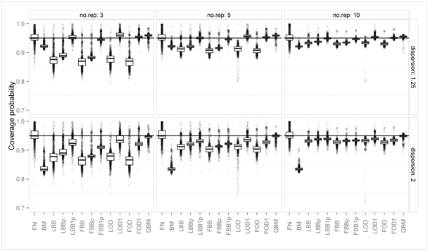
Figure 1 Boxplots of simulated coverage probabilities of nominal two-sided 95% intervals, for different numbers of replications (no.rep) and two different levels of overdispersion.

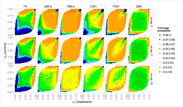
Figure 2 Simulated coverage probabilities (color scale) of nominal two-sided 95% intervals over a grid of true proportions π0, π1, for two-fold overdispersion (ϕ = 2) and nij = 10 biological units in each experimental unit.

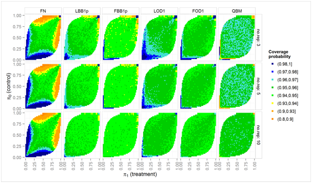
Figure 3 Simulated coverage probabilities (color scale) of nominal two-sided 95% intervals over a grid of true proportions π0, π1, for moderate overdispersion (ϕ = 1.25) and nij = 20 biological units in each experimental unit.

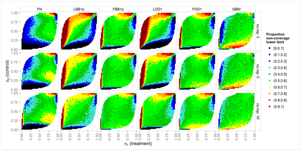
Figure 4 Asymmetry of non-coverage: color scale shows the proportion of cases where the true parameter is excluded by the lower limit all cases where the parameter is excluded by nominal two-sided 95% intervals over a grid of true prop proportions π0, π1, for clear overdispersion (ϕ = 2) and nij = 10 biological units in each experimental unit.

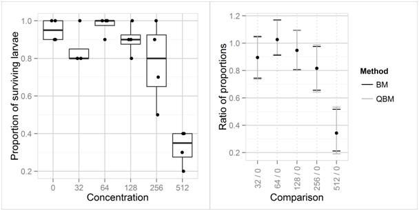
Figure 5 Boxplots and observed proportions of surviving fathead minnow larvae per tank, for the untreated control group and 5 concentrations (left), and 95% confidence intervals of the proportions of surviving larvae in the treatment groups relative to the control group (right)

Results and discussion

Coverage probability of two-sided 95% confidence intervals
Figure 1 shows the simulated coverage probabilities of all 13 methods under comparison: the NF method can either show too low or too high coverage probability, irrespective of increasing sample size, because the relation of mean and variance in the binomial data is ignored. However, its average coverage probability is closer to the nominal level than some of those methods which explicitly account for over dispersed binomial data (LBB, FBB, LBBp, FBBp, LOD and FOD). Simply ignoring the possibility of overdispersion and assuming the binomial distribution results in too low coverage probability even for moderate (1.25-fold) overdispersion: BM method has too low coverage probabilities in nearly all settings. For very small numbers of replications (Ji=3, 5), the far too low coverage probability of the asymptotic methods for overdispersed binomial data (LBB, FBB, LOD, FBB) can be improved slightly by using a pooled variance estimator (LBBp, FBBp) and can be largely improved by setting a lower limit to their variance estimators: If we replace variance estimates suggesting under dispersion by the corresponding estimates under the binomial assumptions, the coverage probabilities of these methods are much closer to the nominal level. The QBM method is always very close to nominal coverage probability but can have slightly too high average coverage probability when overdispersion is moderate and the number of replications is small.

Figures 2 and Figure 3 shows a detailed view on the coverage probabilities in dependence on the true underlying proportions, π0 and π1. This detailed view is restricted to those 6 methods which have an average coverage probability close to 0.95. Figure 2 shows the more difficult case with substantial overdispersion (ϕ = 2), and only nij = 10 biological units in each replication. The QBM methods is close to the nominal confidence levels for a wide range of proportions, but can have too low coverage probabilities if at least one of the proportions is close to 0 or 1. The LBB1p and LOD1 methods need more replications to have coverage probabilities close to 0.95 for a similar range of πi, and still are slightly liberal for almost all πi. LBB1p and LOD1 booth have too high coverage probability for πi close to 0 and too low coverage probabilities when πi close to 1. That is test decisions based on these two methods may be conservative if hypotheses are formulated in terms of mortalities which should be low in the control group, but will be liberal when a similar hypothesis is formulated in terms of the proportion of survivors. In this simulation setting, the Fieller-Bailey-type intervals FBB1p and FOD1 have lower coverage probabilities for almost all parameter combinations considered as compared to the LBB1p and LOD1 method, respectively.

Figure 3 shows results for the less problematic case of moderate over dispersion (ϕ = 1.25) and nij = 20 biological units in each experimental unit. The coverage probability of QBM rarely falls below 0.94, but is slightly too large (between 0.96 and 0.97) if there are only 3 or 5 experimental units per treatment. The LBB1p and FOD1 method have again slightly too low coverage probability if any πi is close to 1, and slightly too high coverage probability if any πi is close to 0. The two Fieller-Bailey-type intervals have slightly lower coverage probabilities than their counterparts based on the log-delta-method.

Symmetry of non-coverage
Figure 4 shows the simulated proportion of cases, where the true parameter was excluded by the lower bound, relative to all cases where the parameter was excluded by the interval. For valid one-sided decisions, methods are preferable that exclude the true parameter equally likely by the lower and upper bound, i.e., with probability α/2 for each limit. For brevity, only the challenging setting with nij = 10 and marked over dispersion (ϕ = 2) is shown, while conclusions for the remaining simulation settings are similar: The Fieller-Bailey-type methods (FBB1p and FOD1) show a wider range of parameter settings where probability of parameter exclusion is equal between lower and upper bounds, as compared to the corresponding methods based on the delta methods on the log scale, LBB1p and LOD1. The QBM method shows asymmetric non-coverage for similar parameter settings as do the Fieller-Bailey-type intervals, i.e. when any of the true proportions is close to 0, but is clearly more symmetric than the FBB1p and FOD1 for a wide range of parameter settings where at least one πi is close to 1.

Examples
Extreme cases: Table 1 shows four extreme cases: Cases 1 and 2 represent cases where proportions are close to 0 in the control treatment as could result from testing the ratio of mortality or immobility proportions. Cases 3 and 4 show data that could arise from test systems that assume proportions close to 1 in the control, for example, survival proportions as in the fathead minnow data below.

	Case 1	Case 2	Case 3	Case 4
Method	x0j = (0,0,0,2) x1j = (1,2,5,6) =0.35/0.05=7	x0j = (0,0,1,1) x1j = (1,2,2,4) =0.225/0.05=4.5	x0j = (8,10,10,10) x1j = (6,7,9,9) =0.775/0.95=0.816	x0j=(10,10,10,10) x1j = (9,9,9,10) =0.925/1=0.925
BM	(1.909, 26.2)	(1.15, 17.5)	(0.656, 0.975)	(0.801, 1.028)
FBB	(1.331, 151.9)	(1.45, 19.8)	(0.657, 1.005)	(0.879, 0.997)
FOD	(1.269, 182.6)	(1.41, 21.0)	(0.654, 1.009)	(0.885, 0.990)
FBB1p	(1.290, 190.0)	(1.24, 28.9)	(0.643, 1.022)	(0.851, 1.028)
FOD1	(1.269, 182.6)	(1.14, 36.8)	(0.654, 1.009)	(0.846, 1.033)
QBM	(0.902, 574.1)	(1.24, 27.6)	(0.558, 1.083)	(0.817, 0.998)

Table 1 95% confidence intervals of selected methods for four extreme cases, assuming all nij = 10, and Ji = 4for two treatment groups, i = 0, 1

In cases 1 and 3, data lead to variance estimates exceeding that of the binomial distribution. Then, the BM method leads to shorter intervals than all other methods. In both cases, the QBM as at least slightly wider confidence intervals than the FBB1p and FOD1 method, which might correspond to the observation that these two have too low coverage probability for small samples. In cases 2 and 4, data show a variance below that of the binomial variance. Then the methods without restriction of variance estimates to that assumed by the binomial distribution (FOD and FBB) yield considerably shorter intervals, than methods which assume that under dispersion is implausible like BM, FBB1p, FOD1 and QBM.

Fathead minnow data: The toxicity of a compound to fathead minnow larvae was investigated using an untreated control group and 5 concentrations of a compound.¹⁶ The experiment comprised 24 tanks, 4 tanks in each treatment group, each tank contained 10 larvae. The observed proportions of surviving larvae are shown in (Figure 5, left side). Analyzing the data in a generalized linear model with quasibinomial assumption, logit link shows that there are highly significant differences between the mean proportion of surviving larvae between the treatments (p < 0.0001; F-test in analysis of deviance). An estimated dispersion parameter of 1.082 suggests that the observations are at most slightly overdispersed, i.e., the data are at least roughly in line with the binomial assumption. The right side of Figure 5 shows two-sided 95% confidence intervals for ratios of the proportion of surviving larvae in the treatment groups relative to that in concentration 0. In this case, confidence limits based on the quasibinomial assumption (QBM) based on the full data including all 6 treatment groups and confidence intervals under the binomial assumption (MOVER-R method for Wilson-Score intervals, BM) do hardly differ.

Conclusion

Asymptotic methods based on the delta method applied on the log-scale or Fieller-Bailey type intervals have too low coverage probabilities when applied in small sample settings that are typical for many bioassays, i.e., they cover the true ratio of proportions less often than claimed by their nominal confidence level. Violation of the nominal level is most severe for small numbers of replications, low number of biological units in each replications and extreme proportions. Even for as much as 10 replications (i.e., clusters), coverage probabilities are considerably below the nominal level for wide ranges of proportions. When these intervals are then used for decisions in hypothesis tests for equivalence or non-inferiority, erroneous conclusions of equivalence or non-inferiority will occur more often than claimed by the nominal level α of such tests.

For the small number of replications and the small number of biological units per replication that are typical for some bioassays, restricting the variance estimates to that of the binomial variance (i.e., setting the dispersion parameter to 1 if under dispersion is estimated) leads to major improvements of the coverage probabilities. Further improvements can be achieved by combining the MOVER-R method with a profile deviance approach leads to intervals with better coverage probabilities for low sample sizes. However, this approach also shows too low coverage probabilities for small sample sizes and cases where one proportion is very close to 0 or 1. However, the simulation results shown here rely on the simplifying assumption, that there is a common overdispersion factor for the treatments in the experiments. Based on single data sets with few replications per treatment it will be hard to assess whether this assumption is appropriate, or whether different overdispersion factors per treatment group (as are used in the FBB, LBB method, for example) would be more appropriate. For given, highly standardized bioassay, however, available collections of historical data sets could be used to assess the plausibility of the different assumptions concerning distribution and mean-variance dependency and homogeneity or heterogeneity of overdispersion factors among treatment groups.

Bioassays usually involve several dosages. Depending on the global hypotheses to be tested, adjustments for multiple comparisons may be needed, see, e.g.¹⁷ The methods for confidence intervals discussed here can be extended to construct approximate simultaneous confidence intervals, using approaches as described in.^17-20 However, such extensions require additional investigation as some approaches involve additional approximations. This is subject to further research.

References

1. Denton DL, Diamond J, Zheng L. Test of significant toxicity: a statistical application for assessing whether an effluent or site water is truly toxic. Environ Toxicol Chem. 2011;30(5):1117‒1126.
2. Lui KL, Mayer JA, Eckhardt L. Confidence intervals for the risk ratio under cluster sampling based on the beta-binomial model. Stat Med. 2000;19(21):2933‒2942.
3. Zaihra T, Paul S. Interval Estimation of Some Epidemiological Measures of Association. Int J Biostat. 2010;6(1):35.
4. Hauck WW, Donner A. Wald's Test as Applied to Hypotheses in Logit Analysis. J Amer Statist Assoc. 1977;72(360):851‒853.
5. Venables WN, Ripley BD. Modern applied statistics with S. 4th edn. New York, USA. Springer-Verlag Inc; 2002:197‒210.
6. Chen JS, Jennrich RI. The Signed Root Deviance Profile and Confidence Intervals in Maximum Likelihood Analysis. J Amer Statist Assoc. 1996;91(435):993‒998.
7. Donner A, Zou GY. Closed-form confidence intervals for functions of the normal mean and standard deviation. Stat Methods Med Res. 2012;21(4):347‒359.
8. McCullagh P, Nelder JA. Generalized linear models. 2nd edn. USA. Chapman & Hall/CRC;1989:124‒135.
9. Johnson NL, Kotz S, Kemp AW. Univariate discrete distributions. 2nd edn. New York, USA. John Wiley & Sons; 1993:239‒284.
10. Fieller EC. Some problems in interval estimation. J Roy Statist Soc Ser B-Stat Methodol. 1954;16(2):175‒185.
11. Fagerland MW, Newcombe RG. Confidence intervals for odds ratio and relative risk based on the inverse hyperbolic sine transformation. Stat Med. 2013;32(16):2823‒2836.
12. Bailey BJR. Confidence limits to the risk ratio. Biometrics. 1987;43(1):201‒205.
13.  Gerhard D. mcprofile: Multiple Contrast Profiles. R package version 0.1-5. 2013.
14. R Core Team. R: A language and environment for statistical computing. Vienna, Austria; 2014.
15. Schaarschmidt F, Gerhard D. pairwiseCI: Confidence Intervals for Two Sample Comparisons. R package version 0.1-25. 2015.
16. Anonymous. Methods for Measuring the Acute Toxicity of Effluents and Receiving Waters to Freshwater and Marine Organisms. 5th edn. U.S. Washington, DC, USA. Environmental Protection Agency; 2002.
17. Hothorn LA, Hasler M. Proof of hazard and proof of safety in toxicological studies using simultaneous confidence intervals for differences and ratios to control. J Biopharm Statist. 2008;18(5): 915‒933.
18. Hothorn T, Bretz F, Westfall P. Simultaneous Inference in General Parametric Models. Biom J. 2008;50(3): 346‒363.
19. Lauzon C, Caffo B. Easy Multiplicity Control in Equivalence Testing Using Two Onesided Tests. Am Stat. 2009;63(2):147‒154.
20. Dilba G, Bretz F, Guiard V. Simultaneous confidence sets and confidence intervals for multiple ratios. J Statist Plann Inference. 2006;136(8):2640‒2658.
Creative Commons Attribution License
©2015 Schaarschmidt. This is an open access article distributed under the terms of the, which permits unrestricted use, distribution, and build upon your work non-commercially.