The oscillation symmetry is applied to several exoplanet masses, quasars, binary neutron stars, and black holes in binary stellar systems. All studied data oscillate clearly and are well fitted with a simple cosine function. The same shape of mass oscillations is observed for different families, the masses of each familly being normalized by the same factor, showing a similarity between these shapes. Thus it is observed, for example, for a planet mass oscillation shape and fundamental particle mass oscillation shape, an oscillation period ratio between both families larger than 10⁵⁵.

The oscillation symmetry, was extended recently, from the classical world to the quantic one varenna. As do the oscillating bodies in classical physics, it was observed that the masses of different members of quantic families oscillate, provided they are subject to opposite interactions. This was observed for hadrons containing quarks, and nuclei excited states made of nucleons. Since these bodies do not merge, neither disintegrate, they are submitted to opposite forces. Indeed the Schrodinger equation contains two opposite forces: kinetic and potential. The oscillation symmetry was also observed for many astrophysical bodies submitted likewise to gravitational forces and centrifugal forces related to their kinetic energies. This symmetry was applied paij paij2 to tentatively predict some properties like for example the putative ninth and tenth new solar planets. The present paper studies different astrophysical bodies, mainly exoplanets. The studied masses are classified in increasing order. The possible oscillations in the mass spectra are studied using the following relation:

$m_{(n+1)}-m_n=f[(m_{(n+1)}+m_n)/2]$                    (1)

where n indicates the increasing mass number, therefore $m_{(n+1)}$  corresponds to the (n+1) mass value. Two successive mass differences are therefore plotted versus their corresponding mean values. This representation is named "mass data" in what follows. A normalised cosine function is used for the fits of the data:^1–3

$\Delta M=\alpha (1+\cos ((M-M_0)/M_1))*\exp (\beta .(M-M_C))$                   (2)

where M/M is defined within 2$\pi$ . The oscillation period is P = 2$\pi M_1$ .

Although there is no clear justification to observe oscillations concerning different properties like the radii of particles, or their orbital oscillations, it was already shown that they are also observed for other properties than masses. The oscillations will be therefore looked for in some figures showing these properties. Thus in equation (2) $\Delta$ M corresponds to the ordinate and M to the abscissa. When fitting the "mass data", $\Delta$ M corresponds to m(n+1) - m(n) and M corresponds to (m(n+1) + m(n))/2. For the other figures M corresponds to the ordinate, and M to the abscissa. M is the variable,$\alpha$ ,$\beta$ , $M_C$  and $M_1$  are the fitted parameters. M₀ is arbitrary and taken to 0. In case of large masses M, a mass $M_c$ is sometimes introduced in order to replace $\beta$ M by $\beta$ $\left(M-M_c\right)$ and avoid a very small $\beta$  value. These $M_c$ are arbitrary and are not therefore considered as a fitted parameter. They are however given in Table A1–A3 since they are bound to the corresponding $\beta$ . The parameters extracted from the fits, are given in Table A1–A3. The fundamental particle masses.⁴ The attempt to predict some properties of the ninth and tenth new solar planets,⁵ has been presented.³

The TRAPPIST-1 exoplanet data⁶ were already discussed in² order to tentatively predict the seventh planet possible mass, unknown at that time. New masses for TRAPPIST-1 exoplanet data are taken from grimm wikitra. The previously six reported masses, in increasing order and in Earth mass unit, are: 0.41, 0.62, 0.68, 0.85, 1.34, and 1.38.² The seven new mass values, in increasing order and in Earth mass unit, are: 0.297, 0.331, 0.772, 0.934, 1.017, 1.148, and 1.156 grimm wikitra. The orbital periods values are not modified. The radii values are almost the same, given the imprecisions. Their new values, in Earth radius unit are: 0.772, 0.918, 1.045, 1.086, 1.127, and 0.775. Figure 1 shows the result of the oscillation symmetry applied to the new data. The four inserts in Figure 1 show successively in the Earth units, for the TRAPPIST-1 exoplanets: the "mass data", the masses versus their orbital periods, versus their radii, and versus their eccentricities. Several other exoplanets masses are studied within the oscillation symmetry. I select the data containing six (sometimes five) such planets around the same star.^9,10

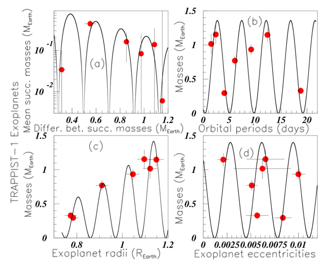
Figure 1 Color on line. (See text). Inserts (a), (b), (c), and (d) show, in the Earth units for the TRAPPIST-1 exoplanets: the "mass data", the masses versus the orbital periods, the masses versus the radii, and the masses versus the eccentricities, respectively.

Figure 2 shows the data and fits of the K2-138 system exoplanet.⁹ Inserts (a), (b), (c), and (d) show respectively (in Jupiter mass units), "mass data", period (in days) versus masses, radii (in Jupiter radius units) versus masses, and "a" the semi-major axis length (in "au": astronomical length units) versus masses. The data of the Kepler-292 exoplanets are taken from⁹ hzq and shown in Figure 3. Their masses are not given. Inserts (a) and (b) show respectively the periods (in days) versus the radii (in Jupiter radius units), and the semi-major axis "a" (in "au" units) versus the corresponding radii (in Jupiter radius units). The data of the HD 10180 exoplanets are taken from¹⁰ and shown in Figure 4(A–C). The orbital periods (in days), the eccentricities and the semi-major axis (in au) versus the planet masses (in Jupiter mass units) are shown respectively in inserts (a), (b), and (c). Insert (d) shows the periods (in days) of the GJ 667 C exoplanets versus their masses hzq. The data of Kepler-20 exoplanets exo, in Jupiter units, are shown in Figure 5. The first four inserts show the data versus the masses. The two last inserts show the data versus the radii.

Figure 2 Color on line. (See text). Inserts (a), (b), (c), and (d) show the “mass data”, the periods versus the masses, the radii versus the masses, and “a” versus the masses of the K2-138 system exoplanets.

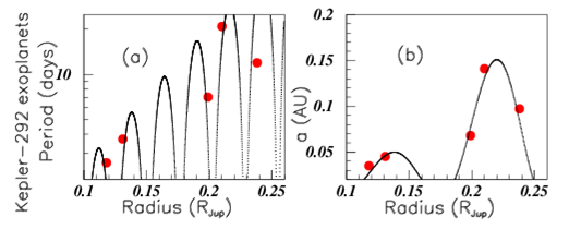
Figure 3 Color on line. (See text). Inserts (a) and (b) show for the Kepler-292 exoplanets, the orbital periods and the semi-major axis length "a" (in astronomic units) versus their radii.

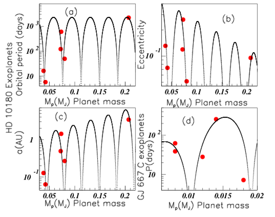
Figure 4 Color on line. (See text). The orbital periods, the ec-centricities and the semi-major axis of the HD 10180 exoplanets, are shown versus the corresponding exoplanet masses, re-spectively in inserts (a), (b), and (c). Insert (d) shows the periods of the GJ 667 C exoplanets versus their masses.

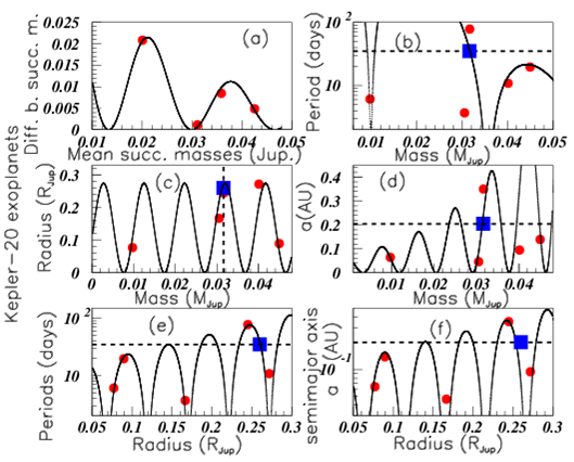
Figure 5 Color on line. (See text). The six inserts show respectively the Kepler-20 exoplanet data in full red circles: "mass data", orbital periods versus masses, radii versus masses, semi-major axis versus masses, periods versus radii, and semi-major axis versus radii. Full blue squares show the sixth planet predicted values for mass and radius.

Five data only are reported for the masses and radii of these exoplanets, but six data are reported for periods and semi-major axis, allowing the use of the oscillation symmetry to tentatively predict the mass and radius of the sixth exoplanet. The period of the sixth data P=34.94 days, shown by a dashed line in insert (b), leads to three possible masses: M0.0091, 0.0107, and 0.0317 M(_Jup). In the same way, the possible masses from insert (d), using the semi-major axis of the sixth planet a=0.2055, are among others: M0.0264, 0.0315, and 0.0360 M(_Jup).

M0.0316 M(_Jup) (M10 M) is therefore the predicted possible mass value of the sixth exoplanet of the Kepler-20 system. However, since the variation of the orbital period data is rather close to that of the semi-major axis data, such determination does not result from an overlap of two different measurements.

Insert (e) shows the Kepler-20 exoplanet orbital periods versus their radii. The possible radii found from insert (e) are: R=0.282, 0.26, 0.234, 0.206, and 0.187 (R_Jup). The same attempt using the semi major axis data "a", shown in insert (f), is again rather meaningless since their is no large variation between the ratios of orbital periods versus "a". Indeed the radii extracted from the insert (f) can be: r=0.279, 0.254, 0.2304, 0.200, and 0.183 R_Jup. From insert (c) we are able to conclude that, when using the mass possible value M0.0316 M(_Jup) the possible radius might be R0.26 R_Jup. These values are reported in Figure 5 by blue squares.

Figure 6 shows data of the Kepler-33 five exoplanets exo. Note that different values of Kepler-33 exoplanet data are given in hzq. Inserts (a) and (b) show the periods (in days) and semi-major axis (in au) versus the explanet radii (in R). Inserts (c) and (d) show the same data versus the inclination (in degrees) where only four "i" data are given. The period value (P=41.029 days) suggests two possible values for "i": 89.7 or 89.97 degrees. The "a" value (a=0.2535 ua) suggests for "i": 89.73 or 89.93 degrees. The oscillation symmetry allows therefore to sugest i89.8 degrees for this missing value. Figure 7 shows the data of the six HD 34445 exoplanets hzq. Inserts (a), (b), (c), and (d) show respectively the "mass data", the orbital periods then eccentricities versus masses, and the periods versus the eccentricities. Figure 8 shows the HD 219134 exoplanet data hzq. Insert (a), (b), and (c) show the "mass data", the orbital periods (in days) versus the masses (in Jupiter masses), and the eccentricities versus the masses. Six values are known for these data. Insert (d) shows the masses versus the radii (in Jupiter unit radii). Only four radii are known for this exoplanets. The masses without known radius are marked by horizontal dashed lines. They are M=0.034 M_Jup and M=0.034 M_Jup. It is not possible to propose a radius corresponding to M=0.034 M_Jup since the corresponding line intercepts many times the fit. On the other hand the oscillation symmetry allows to suggest the radius M0.156 R_Jup for the planet with mass M=0.34 M_Jup. But due to the very low number of data available for the fit, this last suggestion is more uncertain than the previous ones. Figure 9 shows the orbital periods (in days) plotted versus the radii (in R_Jup) hzq, respectively in inserts (a), (b), (c), and (d), for the following exoplanets: KOI-351, Kepler-80, Kepler-186 and Kepler-296.

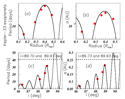
Figure 6 Color on line. (See text). The Kepler-33 exoplanet data are studied. The orbital periods and semi-major axis are plotted versus the radius in inserts (a) and (b) and versus the inclination in inserts (c) and (d).

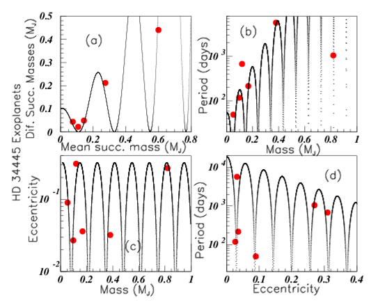
Figure 7 Color on line. (See text).The exoplanet HD 34445 data are shown in the four inserts: "mass data", orbital periods versus masses, eccentricities versus masses, and orbital periods versus eccentricities.

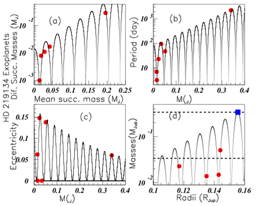
Figure 8 Color on line. (See text).Inserts (a), (b), (c), and (d) show the "mass data", orbital periods versus masses, eccentricities versus masses, and masses versus radii.

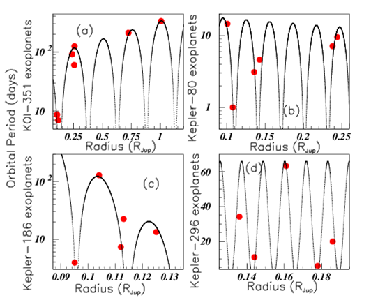
Figure 9 Color on line. (See text). Study of orbital periods versus radii of the following exoplanets: KOI-351, Kepler-351, Kepler-186, and Kepler-296, in inserts (a), (b), (c), and (d) respectively.

The four inserts of Figure 10 show the data for Kepler-11 exoplanets. Inserts (a), (b), (c), and (d) show respectively the differences between successive masses versus their corresponding mean values in Jupiter mass units, the radii (in Jupiter radii units) versus the masses, the orbital periods (in day units) versus the masses, and the eccentricities versus the masses. The three inserts of Figure 11 show several data of the Kepler-90 exoplanets also named KOI-351. The masses and radii are taken from kyoto. The "mass data" (in Jupiter units), the semi-major axis (in (au) units) versus the radii (in Jupiter radii), and the masses versus the orbital periods (in days), are studied respectively in inserts (a), (b), and (c). The large masses and periods of two of these exoplanets are omitted in insert (c) otherwise the other six data would be too tightly packed. Previous figures show the behaviour of several exoplanets spinning around stars. Figure 12(A) shows the exoplanet "mass data" oscillation periods (in M) studied above, versus the corresponding star masses (in solar mass units). Figure 12(B) shows the star radii (in solar radius units) versus the star masses (in sun mass units).

Figure 10 Color on line. (See text). Inserts (a), (b), (c), and (d) show respectively the "mass data", radii, orbital periods, and eccentricities versus the masses of the Kepler-11 exoplanets.

Figure 11 Color on line. (See text). The Kepler-90 exoplanets are studied. Inserts (a), (b), and (c) show in Jupiter units, the "mass data", the semi-major axis versus the radii, and the masses versus the orbital periods.

Figure 12 Color on line. (See text). Insert (a) shows the exoplanet "mass data" oscillation periods (in MJup:) versus the star masses. Insert (b) shows the star radii (in sun radius units) versus the star masses (in sun mass units).

Figure 13 studies the difference of successive redshift "z" z distances of Quasars having quasars versus the mean successive corresponding distances.

Figure 13 Color on line. (See text). Redshifts $z\ge 6$ quasar distances plotted versus their mean successive values.

Figure 14 shows several data corresponding to black holes in binary systems and galactic nuclei cher. All masses are given in solar mass units. Inserts (a), (b), and (c) show respectively the orbital periods of the system (in days) versus the mass functions, the black hole masses mX versus the rotational velocity (in km/s), and the black hole masses versus the star optical masses m. Since the corresponding error bars are large, these data are, as previous data, fitted by the oscillations obtained using relation 1.

Figure 14 Color on line. (See text). Binary black hole systems data. The orbital periods versus the mass functions, the black hole masses versus the rotational velocities, and the black hole masses versus the star optical masses, are shown respectively in inserts (a), (b), and (c).

Figure 15 shows some data of binary neutron stars etneutrons. The companion of the first star is interpreted as being another neutron star. Insert (a) shows the difference between successive binary neutron star total masses versus the corresponding mean successive masses etneutrons, both in solar mass units. Figure 15(B) shows the binary neutron star total masses versus the difference between both masses, in solar mass units (Table 1).

Figure 15 Color on line. (See text). Insert (a) shows the "mass data" of the binary total star masses. Insert (b) shows the total binary star masses versus the mass difference between both compagnon binary star masses.

The "mass data" oscillations are observed in many families such as fundamental particles, mesons, baryons, nuclei excited state levels, and several different astrophysical bodies. Whereas such behaviour may be anticipated for masses resulting from Schrdinger equation, this is not the case for other properties. However this oscillation property seems to be rather general, suggesting therefore to look at possible same, or at least similar behaviours through an homothety allowing to join together different body families. The homothety involves a mass translation and also a change of oscillation period which is multiplied by this factor. Figure 16 shows that the same fit allows to describe the "mass data" of several exoplanet masses, provided they are normalized through a simple homothety. The fit correponds to HD 34445 exoplanet "mass data" shown by full red circles. The Kepler-11 exoplanet "mass data", normalized by the coefficient 22.7, are shown with blue full squares. The K2-138 system exoplanet "mass data", normalized by the coefficient 23.7 are shown with green full triangles. They all are well described by the same fit. Figure 17(A) shows the periods (in days) versus the masses (in Jupiter masses) for the HD-34445 Exoplanets in full red circles, fitted by the drawn curve, and HD-219134 Exoplanets in full blue squares, with masses normalized by a factor 3, allowing the agreement with the fit performed on HD-34445 Exoplanet periods. Figure 17(B) shows the periods (in days) versus the masses (in Jupiter masses) for Kepler-20 Exoplanets in full red circles fitted by the drawn curve, and K2-138 Exoplanets in full blue squares, with masses normalized by a factor 2.

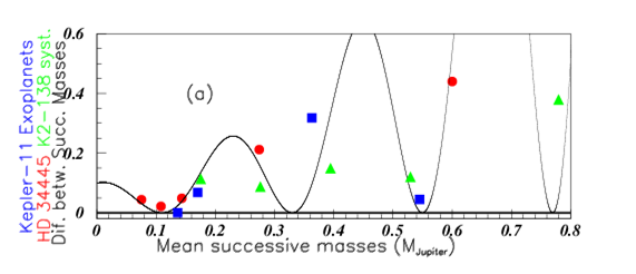
Figure 16 Color on line. (See text). Red full circles show the HD 34445 exoplanet "mass data", blue full squares show the Kepler-11 exoplanet homothetic "mass data", and green tri- angles show the K2-138 system exoplanet homothetic "mass data".

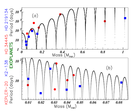
Figure 17 Color on line. (See text). Insert (a) shows the HD 34445 exoplanet periods versus the corresponding masses in red circles and exoplanet HD 219134 homothetic periods versus their masses in blue squares. Insert (b) shows the Kepler -20 exoplanet periods in red circles and K2-138 exoplanet homothetic periods in blue squares.

The previous figures show that the different exoplanet "mass data" display the same oscillating figure, provided that a simple homothetic factor is performed on the masses. With the next figures I am wondering wether this property is still verified for different kind of mass families. Figure 18 shows the mass difference versus the mean corresponding masses for:

1. Solar planets in full red circles, in units of 10²⁴ kg. The two additional possible solar planets⁵ taken into account. It was shown³ that the fit, inside the oscillation symmetry, remains good after these two planets addition. The present fit is performed using these data.
2. Trappist exoplanet masses⁷ blue full squares, in units of 10²⁴ kg multiplied by the homothetic factor 115. Notice that somewhat different masses are given in different publications.
3. Quark masses (in MeV) are plotted with green full upside triangles.
4. Lepton masses (in MeV) are plotted with black full downside triangles.

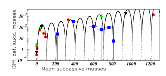
Figure 18 Color on line. (See text). Mass differences versus corresponding mean masses of solar planets (red circles), Trappist exoplanets (blue squares), quarks (green upside tri-angles), and leptons (black downside triangles). The different body family units are explicited in the text.

Figure 19 shows the difference between successive masses versus the corresponding mean values of several different families (the "mass data"):

1. Full blue squares show the f₂ meson "mass data". The fit is performed on these data.
2. Full green stars show the f₀ meson "mass data" with the homothetic factor: 0.7.
3. Full red circles show the baryon "mass data" with an homothetic factor: 0.94.
4. Full upside purple triangles show the baryon "mass data" with an homothetic factor: 0.91.
5. Black empty star inside empty squares show the ¹⁴N excited state levels modified by the homothetic factor: 114.

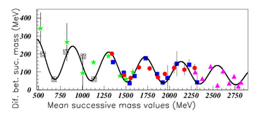
Figure 19 Color on line. (See text). Comparison of "mass data" between several families. essai1254.eps fas19.eps.

The fit here is obtained with a relation which uses four parameters (since =-0.0035 and Mc=200 are correlated):

y=(120*cos(M/66)+190)*exp(-0.0035*(M-200)). A single fit describes nearly all data since two data only are outside the fit. Figure 20(A) shows the difference between the hadronic masses (in MeV) versus their corresponding mean masses (in MeV) of:

1. N (1/2) in full red circles,
2. N (3/2) in full blue circles,
3. (1/2) in full green stars, and
4. (3/2) in empty purple stars surrounded by empty square.

All these data are well fitted by a unique distribution. Figure 20(B) shows the total widths (in MeV) of the same baryons and same marks as in (a), plotted versus their masses, and well fitted with a single distribution. There is no homothetic factor on masses, neither in figure 20(a) nor in Figure 20(B) (Table 3).  and P are in MeV.  are in MeV^-1. When not given, the homothetic factors=1. See text.

Figure 20 Color on line. (See text). The baryonic total widths are plotted versus the corresponding masses by: full red circles for N(1/2)*, full blue squares for N(3/2)*, full green stars for (1/2)*, and purple squares for (3/2)*.

The oscillation symmetry is applied to several astrophysical body masses and some other properties. Several exoplanet data are selected when at least five such planet data are reported around the same star. The data exhibit oscillation shapes, well fitted with a simple cosine equation, most often using three parameters. This allowed to tentatively predict some still unknown properties. Although these shapes differ for different data, it is observed that they are often common shapes which can be reduced to the same one provided an homothety is done (mass renormalization). It was first shown for several exoplanet "mass data" shapes. It was also shown more generally to very different body families, like exoplanets and fundamental particles. So the drawing look the same, and will infer one from the other by homothety. So it seems that the oscillation symmetry is often observed in nature but the corresponding meaning is unknown (except eventually for masses). In the same way, I do not understand why the same variation, through an homothety, is observed for some data mass shapes.

None.

Author declares that there are no conflicts of interest.

None.

1. B Tatischeff. Oscillation symmetry applied to: 1) hadronic and nuclei masses and widths 2) astrophysics. And used to predict unknown data. Proceedings of the 15 ^th International Conference on Nuclear Reaction Mechanisms, Varenna, Italy, 2018. p. 35.
2. B Tatischeff. May the oscillation symmetry be applied to TRAPPIST-1 terrestrial planets to predict the mass of the seventh planet ? Phys Astron Int J. 2018;2(3):193.
3. B Tatischeff. Oscillation symmetry applied to several astrophysical data. Attempt to predict some properties of the putative ninth and tenth new solar planets. Phys Astron Int J. 2019;3(6):267–274.
4. M Tanabashi. Particle Data Group. Phys Rev D. 2018;98.
5. S Rouat. A la rechrche des planetes Neuf et Dix. Sciences et Avenir. 2017;850:42.
6. M Gillon, AH Triaud, BO Demory, et al. Seven temperate terrestrial planets around the bear by ultra cooldwarf star TRAPPIST-1. Nature. 2017;542(7642):456–460.
7. S Grimm, BO Demory, M Gillon, et al. The nature of the TRAPPIST-1 exoplanets. Astronomy &  Astrophysics. 2018;613(2018)A68.
8. https://fr.wikipedia.org/wiki/TRAPPIST-1
9. www.exoplanet.eu/catalog
10. www.hzgallery.org/table.html
11. www.exoplanetkyoto.org/exohtml/Kepler-90.html  
12. https://en.wikipedia;org/wiki/Distancemeasures(cosmology)
13. https://wikipedia.org:wiki/Listesdequasars
14. AM Cherepashchuk. Black holes in binary stellar systems and galactic nuclei. UFN. 2014;184(4):387.
15. https://fr.wikipedia.org/wiki/EtoileÃneutrons