Several astronomical data are shown to fulfill an oscillatory symmetry. This is the case for very large distance objects as galaxies, but also for objects at relatively small astronomical distance as the solar planet moons and rings. Their masses exhibit oscillatory figures, leading us to tentatively assume to use this oscillatory symmetry to predict still unknown property, namely the mass of the TRAPPIST–1 seventh terrestrial planet.

PACS numbers: 26.00.00 96.15.De 96.20.–n 96.30.–t 96.60.Bn 97.10.Nf

Keywords: planet, oscillation, quantum physics, Schrödinger equation, nuclei, plasmas, centrifugal forces, kinetic energy, gravitation

A few papers have pointed out recently a new property of hadronic masses, and masses of nuclei excited state levels.^1,2 This property was called oscillation symmetry. The hadron family masses and the masses of the excited state nuclei levels showed nice oscillations, provided they were selected for given spins. In classical physics, it is known that two opposite forces create an oscillatory system. The previous observation shows that the same is observed in quantum physics because such situation arises in systems built with sub–systems like nuclei or hadrons. The masses of hadrons or nuclei, solution of the Schrödinger equation, containing two opposite interactions, obey to this classical physical law.

Indeed in these cases, an attractive force holds the sub–systems together, and a repulsive force prevents the sub–systems from self–destruction like plasmas. When referring to masses, I classified them in increasing order, and then investigated the function:

$m_{\mathrm{<mo\; stretchy="false">(</mo>}n+\mathrm{1<mo\; stretchy="false">)</mo>}}-m_n\mathrm{<mo>=</mo>}f\mathrm{<mo\; stretchy="false">[</mo><mo\; stretchy="false">(</mo>}{m}_{\mathrm{<mo\; stretchy="false">(</mo>}n+\mathrm{1<mo\; stretchy="false">)</mo>}}+m_n\mathrm{<mo\; stretchy="false">)</mo><mo>/</mo>2<mo\; stretchy="false">]</mo>}$       (1)

where$m_{\mathrm{<mo\; stretchy="false">(</mo>}n+\mathrm{1<mo\; stretchy="false">)</mo>}}$ corresponds to the$\mathrm{<mo\; stretchy="false">(</mo>}n+\mathrm{1<mo\; stretchy="false">)</mo>}$ mass value. The difference of two successive masses is plotted versus the mean value of these two masses.

Another observation was performed concerning the widths of these hadronic³ and nuclei levels. The widths, plotted versus the corresponding masses, show also oscillatory behaviours although they do not result from the solution of a simple Schrödinger equation, suggesting that this oscillation symmetry may be widely observed in nature.

All the data analyzed below are fitted using a cosine function

$\Delta m\mathrm{<mo>=</mo>}{\alpha }_0+{\alpha }_{1}cos\mathrm{<mo\; stretchy="false">(</mo><mo\; stretchy="false">(</mo>}m-M_0\mathrm{<mo\; stretchy="false">)</mo><mo>/</mo>}{M}_1\mathrm{<mo\; stretchy="false">)</mo>}$        (2)

where$M_0/M_1$ is defined within$2\pi$ . The oscillation periods are$P=2\pi M_1$ . Both${\alpha }_0$ and${\alpha }_1$ are first adjusted in the whole interval, for each figure. The quantitative prediction of the oscillation amplitudes needs theoretical studies, which are outside the scope of the present paper. These amplitudes are not discussed. Whereas smaller periods might fit the data, the following figures correspond to the largest possible values of the periods. All${\alpha }_0$ ,${\alpha }_1$ and P values are reported in Table 3. $M_0$ depends on the origin of the fit, modulo an integer number of periods. In order to illustrate this property, Figure 1 reproduces few examples of the oscillations observed in hadrons⁴ and nuclei.

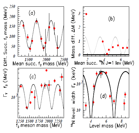
Figure 1 Color on line. the four inserts show the mass differences versus the corresponding mean masses for f₂ mesons in insert (A) and ${}^{16}N$ (J=1) levels in insert (B), and the corresponding total widths of f₂ mesons in insert (C) and widths of the ${}^{16}N$ (J=1) excited levels in insert (D).

Figure 1 shows the mass differences versus the corresponding mean masses for f₂ mesons⁴ in insert (a) and ${}^{16}$ N (J=1) levels⁵ in insert (b), with respective measured periods P=415 MeV and P=1.82 MeV. The corresponding total widths of f₂ mesons (P=358 MeV) and of ${}^{16}$ N (J=1) excited levels (P=3.02 MeV) are shown in inserts (c) and (d). The oscillatory behaviours are obvious. For example in Figure 1A, the fit for a straight line plotted with all the data, gives rise to a normalized ${\chi }_2$ (lin) = 11.0, when the normalized${\chi }_2$ (fit) obtained by using the plotted curve equals 1.07. Many similar studies have been performed.^2,3

The oscillation symmetry was first observed as being an intrinsic property of a body (pendulum or spring ...), submitted to opposite forces, kinetic and potential. Since the nuclear masses are also submitted to opposite kinetic and potential interactions through the Schrödinger equation, it was tempting to investigate possible oscillations inside hadronic and nuclear masses. The corresponding studies showed that this was indeed the case. Such observation corresponds to an extension from one body property to "several body properties", as if they belong to one common entity.

Both one body and "many body" oscillations are the consequence of opposite acting forces. It is therefore well–founded to question about a possible similar observation in the astronomical field. Indeed, here again, all bodies are subjected to interactions acting in opposite ways, being respectively attractive (gravitation) and repulsive (centrifugal forces related to the kinetic energy). Otherwise they would either merge or keep apart for ever.

The applicability of the used method in astronomical researches is based on the following: the previously observed oscillations were evidenced when opposite forces did exist. Indeed, the forces in quantum physics (hadrons and nuclei) are totally different from the forces inducing the pendulum motion. This shows that the oscillations are not connected to the nature of the intrinsic forces. In fact, the oscillations originate from the existence of potential and kinetic interactions. Although astronomical forces are quite different from the previous considered forces, the astronomical bodies are also submitted to opposite forces (repulsive: centrifugal forces related to the kinetic energy, and attractive: gravitation) within which they reach an equilibrium. It is a reason to investigate, by using published data in the field, whether astronomical bodies might depict a similar oscillatory behaviour. I first focused on the moons and on the ring widths of solar planets.

Figure 2 shows, in log scale, the diameters of two solar planet moons (in km),⁶ Saturn in insert (a) ($P=79.2*{10}^{3}km$ ), and Uranus in insert (b) ($P=21.4*{10}^{3}km$ ), plotted versus their distances from their respective Solar planets (in ${10}^3$  km units). Only the data corresponding to distances smaller than 600,000 km from Saturn are kept in the Figure 2A. In the same way, only data correponding to distances lower than 200,000 km from Uranus, are kept in Figure 2B. The diameter period is larger for Saturn planet moon oscillations, compared to Uranus planet moon oscillations.

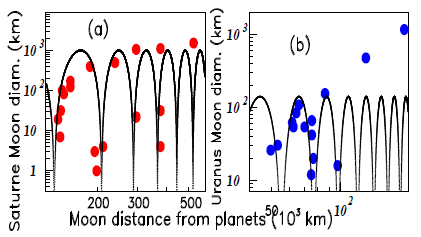
Figure 2 Color on line. saturn moon diameters in insert (A) and uranus moon diameters in insert (B) plotted versus their respective distances from the planet.

Figure 3 shows the ring widths (in km) of the Solar planets Saturn (a), Uranus (b), and Neptune (c) plotted versus each Solar planet mean radius (in ${10}^3$  km). The fitted period P of each Solar planet ring oscillations, divided by the already known Solar planet mean radius "r", is more or less constant (Table 1).

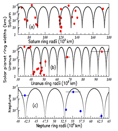
Figure 3 Color on line. saturn, uranus, and neptune ring widths plotted versus the corresponding planet ring radii.

The log scale in y axis of Figure 2 & 3, is appropriate for fitting with the used function.

The data plotted above (Figure 2 & 3), show that the oscillation symmetry is still observed in different astronomical data. This allows us to use this property to tentatively predict some missing information. Therefore, I have chosen to question the unknown mass of the seventh terrestrial planet recently evidenced around the TRAPPIST–1 star. Seven temperate terrestrial planets have been observed around the star TRAPPIST–1.^7–9 Different properties are given for all of them, except the mass (and therefore the density) for the seventh planet called "h".^7–9 The oscillatory symmetry method is applied to tentatively predict the missing mass of the seventh planet. . The large mass inaccuracy of the six known TRAPPIST–1 terrestrial planet masses, involves poor precision for the fits. First, in order to increase the proof of the general oscillatory property, I start to show in Figure 4 several more precise properties of these planets, plotted versus other precise properties of the same planets.

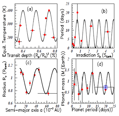
Figure 4 Color on line. the figure shows in inserts (A), (B), and (C) respectively, the galaxy brightenesses, the galaxy masses, and the diameters of the milky way satellite galaxies versus their distances from earth. Arrows and dashed lines (in inserts (A) and (B)) show the assumed possible positions of two yet unobserved galaxies.

Figure 4 shows the following TRAPPIST–1 planet properties in the following four inserts: the equilibrium temperature in (K) versus the transit depth${(R_p/R_0)}^2$ (%) in insert (a) (P=0.164 units), the orbital periods (in days) versus the irradiation$S_p$ in ($S_{Earth}$ ) in insert (b) (P=0.861 units), the radius $R_p$  in ($R_{Earth}$  units) versus the semi–major axis (in${10}^{-3}$ AU units) in insert (c) (P=33.0 units), and finally the planet masses in ($M_{Earth}$ units) versus the planet orbital periods in (days) in insert (d) (P=4.78 days). The squares in Figure 4D shows the possible seventh’s planet mass, which value will be determined later as being the mean value of the masses suggested through extraction from other variables (see below).

Figure 5 shows in the four inserts the plots of the TRAPPIST–1 planet masses (in Earth mass units): (a) versus their radius (in Earth radius units) (P=0.251 units), (b) versus the transit impact parameter (in Solar radius units) (P=0.251 units), (c) versus the equil.ibrium temperature (in Kelvin’s units) (P=144.5 units), and (d) versus the scale parameter (in$a/R{ }_0$ units) (P=81.7 units). "a" is the semi–major axis and R the Solar radius. The blue vertical dashed lines show the range value of the seventh’s planet data determined by the uncertainty on the known data plotted in the abscissa. The blue stars surrounded by squares show our prediction on the possible seventh planet mass and its uncertainties. Figure 2A of^7–9 and the radius of the seventh planet, imply that the mass of this planet has to be lower than 0.75 times the earth mass, otherwise the composition of the seventh planet will exceed 100% iron. That helps to drive the fits.

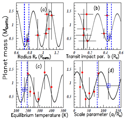
Figure 5 Color on line. the data correspond to TRAPPIST–1 terrestrial planets. Inserts (A–D) show the equilibrium temperatures versus the transit depths (A), the orbital periods versus the irradiations (B), the radii versus the semi–major axis "a" (C), and the planet masses versus the planet orbital periods (D). The square shows the possible mass of the seventh planet (see text).

Figure 6 shows the plots of the TRAPPIST–1 terrestrial planet masses (in Earth mass units) (a) versus the irradiation$S_p$ (in$S_{EARTH}$ ) (P=2.26 units); (b), versus the transit duration time W (in min) (P=30.2 min), (c) versus the semi–major axis, "a" (in${10}^{-3}$ AU) (P= 25.8 units), and (d) versus the transit depth${(R_p/R_0)}^2$ (%) (P=0.295 units). As in Figure 5, the fits are obtained by using the data from the six planets with known masses. The blue vertical dashed lines show again the range value of the seventh planet, and the blue stars surrounded by squares the possible seventh planet mass. The unknown mass is badly determined from the data of Figure 6C.

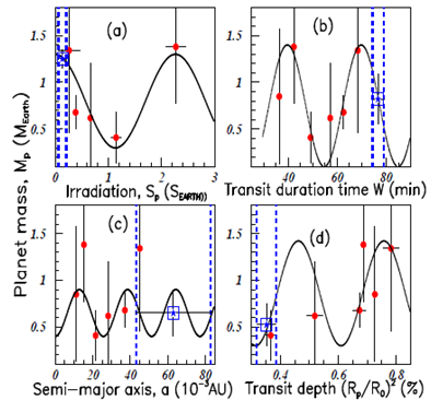
Figure 6 Color on line. the data correspond to TRAPPIST–1 terrestrial planet properties. Inserts (A–D) show the data of the six planet masses versus: their radii (A), their transit impact parameters (B), their equilibrium temperatures (C), and their scale parameters (D). The square shows the possible seventh planet mass (see text).

The characteristics of the fits in Figure 5 & Figure 6 are shown in Table 2. The fits are significant when the blue data is located close to a known data (a red data), as in Figure 5A, Figure 6A & Figure 6D. The oscillatory periods are also shown in the Table 2.

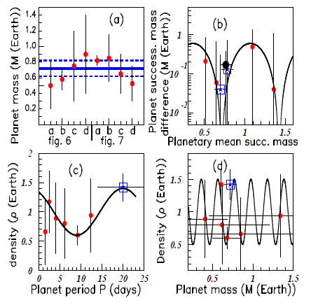
Figure 7 shows in insert (a) the various masses of the seventh planet, extracted from Figures 5 & Figure 6. The mass error bars are obtained using the fits and the mass error bars of the fitted data (radius, transit impact parameter, ....), that is to say from the intersection of the dashed blue vertical lines with the graphs. The obtained mass mean value of the TRAPPIST–1 seventh planet is$M\left(7\right)\approx 0.72\pm 0.07$ (in Earth mass units). Its precision does not take into account systematic effects due to the choice of the fit function. Therefore the unprecision of this prediction may be larger, and is increased up to 0.1. The planet density$\rho$ , corresponding to$M\left(7\right)\approx 0.7\pm 0.1$ (in
Earth mass units), is then$\rho \approx 9.1\pm 1.3 {\text{g/cm}}^3$ .

Figure 7 Color on line.inserts (A–D) show the data of the six known TRAPPIST–1 planet masses versus: their irradiations (A), their transit duration times (B), their semi–major axis (C), and their transit depths (D). The square corresponds to the seventh planet (see text).

After classifying the mass of the seven planets in increasing order, Figure 7B shows, according to Equation (1), the successive mass difference (in$M_{Earth}$ units) plotted versus the corresponding mean mass value. The period here is (P=0.71 M). Two data points, drawn by blue stars surrounded by squares, show the new data obtained when the seventh planet mass is introduced. Figure 7C shows the densities in (${\rho }_{Earth}$ ) units versus the planet orbital periods in ($P_{days}$ ) units (P=22 days).

Figure 7D shows the planet densities$\approx 0.72\pm 0.07$  (in Earth mass units) in (${\rho }_{Earth}$ ) units versus the planet masses in ($M_{Earth}$ ) units (P=0.204 units). The new data, by taking into account the seventh planet, agree very well with the fits of the three inserts (b), (c), and (d).

The paper shows that the discussed data follow oscillatory behaviours. The forces acting in our daily world on pendulums or springs are very different from forces involved in quantum physics on hadrons, or nuclei. In both cases, oscillations are observed. In each field, they are always induced by the existence, of opposite forces, having the same order of magnitude. The forces acting in the astronomic field are very different from the previous ones, but again, the presence of opposite interactions induces the observed oscillations. This is shown to be the case for Saturn and Uranus moon diameters plotted versus the moon distances from planets, and for Saturn, Uranus and Neptune ring widths plotted versus the corresponding planet ring radii.

The variation of several precise data (except masses) corresponding to the seven planets around Trappist–1 star, are studied in the first three inserts of Figure 4. They all show oscillatory behaviors.

Therefore, the oscillation symmetry applies well for astronomical bodies as well as for classical and quantum bodies, als–l terpla*l though these bodies are submitted to different forces. I have used that property to tentatively predict the mass of the seventh TRAPPIST–1 terrestrial planet:$M\left(7\right)\approx 0.7\pm 0.1$ (in Earth mass units). A verification of the applicability of the used method would be the measurement of this mass, with its presumed order of magnitude. This method can be applied to a large number of physical problems, provided that the conditions of oscillation symmetry exist. Such studies can be fullfilled if several data exist per arch of oscillation, an essential condition for determining the oscillating periods.

None.

Author declares there is no conflict of interest.

1. Tatischeff B. Systematics of oscillatory behavior in hadronic masses and widths. USA: Cornell University Library. 2016. p. 1–5.
2. Tatischeff B. Variation of hadronic and nuclei mass level oscillation periods for different spins. Journal of Particle Physics. 2017;1(1):13–29.
3. Tatischeff B. Oscillation symmetry applied to nuclear level widths and masses. Journal of Particle Physics. 2018;2(2):5–22.
4. Olive KA. Review of Particle Physics. Chinese Physics C. 2014;38(9).
5. Tilley DR, Weller HR, Cheves CM. Energy Levels of Light Nuclei A=16. Nuclear Physics A. 1993;564(1):1–174.
6. https://www.windows2.universe.org/our solar system/moons table.html
7. https://fr.wikipedia.org/wiki/Groupe_local
8. https://en.wikipedia.org/wiki/Milky_Way
9. https://en.wikipedia.org/wiki/Satellite_galaxies_of_the_Milky–Way

References

Creative Commons Attribution License
©2018 Tatischeff. This is an open access article distributed under the terms of the, which permits unrestricted use, distribution, and build upon your work non-commercially.