Oscillation symmetry applied to several astrophysical data. Attempt to predict some properties of the putative ninth and tenth new solar planets

doi:10.15406/paij.2019.03.00193

eISSN: 2576-4543

Physics & Astronomy International Journal

Mini Review Volume 3 Issue 6

Oscillation symmetry applied to several astrophysical data. Attempt to predict some properties of the putative ninth and tenth new solar planets

B Tatischeff

Verify Captcha

Regret for the inconvenience: we are taking measures to prevent fraudulent form submissions by extractors and page crawlers. Please type the correct Captcha word to see email ID.

Université Paris-Saclay, France

Correspondence: B Tatischeff, Universite Paris-Sud, Université Paris-Saclay, IPNO, CNRS/IN2P3, 91406 Orsay Cedex, France, Tel +3316 9155 172

Received: November 15, 2019 | Published: December 3, 2019

Citation: Tatischeff B. Oscillation symmetry applied to several astrophysical data. attempt to predict some properties of the putative ninth and tenth new solar planets. Phys Astron Int J. 2019;3(6):267-274. DOI: 10.15406/paij.2019.03.00193

Download PDF

Abstract

The existence of opposite forces acting on astrophysical bodies, involve that their properties should obey to oscillation symmetry. The oscillation symmetry is applied to several astrophysical properties, like Nebulae radii and magnitudes, Local Group Galaxy masses, luminosities, and diameters, Comet radii, orbital periods, and eccentricities, Black hole masses, orbital periods, and distance from earth, Star masses, magnitudes, and distances from Sun. This symmetry is used to predict some still unknown astronomical properties, namely the properties of two additional possible solar planets. Using the predicted possible masses of these planets the method allows to predict their possible densities, rotation durations, revolution periods, orbital speeds, and eccentricities.

PACS numbers: 26.00.00 96.15. De 96.20.-n 96.30.-t 96.60.Bn 97.10.Nf.

Keywords:oscillation, symmetry, astrophysics, solar planets, galaxies, comets, black holes, stars

Introduction

It was recently highlighted that the oscillation symmetry applies not only on the classical world, but also on the quantum one, provided that the studied objects are submitted to opposite interactions. This method was applied to hadron masses and widths and to masses and widths of some nuclei excited levels.¹ Since the interactions involved in classical and quantum worlds are very diﬀerent, it was concluded that this property depends on the existence of opposite forces acting on the studied bodies, and not on the nature of the interactions involved.This is also the case for astronomical bodies as - for example - planets turning around stars, since they are submitted to gravitational forces and centrifugal forces related to the kinetic energy. The oscillation symmetry method was used to show the oscillations of Saturn and Uranus moon diameters versus the moon distances from planets,² and the Saturn, Uranus, and Neptune ring widths versus the same planet ring radii. It was also used to study the possible mass of the seventh’s planet² turning around the dwarf star TRAPPIST-1.³

Some results concerning hadron physics and nuclear physics have already been published,⁴ but with a somewhat diﬀerent relation used to ﬁt the data (see below). The present paper studies the oscillations in several astrophysical data: Nebulae, Black holes, Local group Galaxies, Comets, Stars, Supernovae, Pulsars, and Solar planets. The present paper studies also some possible properties of the predicted ninth and tenth new solar possible planets.⁵ The existence of the ninth planet mass was postulated in order to explain the strange behavior of some bodies belonging to the Kuiper’s belt.⁶ The authors concluded that the mass of the ninth giant planet should be e.m. (earth mass). In the following, I will consider this mass as being In order to understand the abnormal behavior of Kuiper’s belt bodies and the Kuiper’s cliﬀ, diﬀerent authors suggested the existence of a tenth planet with a mas ⁷Since the existence of these two new solar planets remains controversial, the oscillation symmetry approach is applied to the solar planet masses in order to see if the new masses agree - or not - with the masses of the eight ”classical” solar planets ?

The oscillation symmetry

The studied masses are classiﬁed in increasing order, then the possible oscillations in the mass spectra are studied using the following function:

$m_{(n + 1)} - m_{n} = f [(m_{(n + 1)} + m_{n}) / 2]$ (1)

$m_{(n + 1)}$ corresponds to the (n+1) hadron mass value. Two successive mass diﬀerences are therefore plotted versus their corresponding mean masses.

A normalized cosine function is used for the ﬁts:

$Δ M = α (1 + \cos ((M - M_{0}) / M_{1})) * e^{β . M}$ (2)

where $M / M^{1}$ is deﬁned within $2 π .$ The oscillation periods, $P= 2 π M_{1}$ are studied. The amplitude of oscillations deserves theoretical studies which are outside the scope of the present work. M⁰ depends on the mass chosen to start the ﬁts, and is therefore arbitrary, and taken as zero. The ﬁts are obtained with two parameters when the oscillation amplitudes are constant $(β = 0),$ and three parameters when the oscillation amplitudes move progressively with a multiplicative value $e^{β . M} .$ The parameters used for the ﬁts are given in Table 1. In this table the units for α are those of the ordinate, the units of β are the inverse of the abscissa units (the inverse of the period unit). The formula used previously, to be compared to (2), was:

$Δ M = α_{0} + α_{1} \cos ((M - M_{0}) / M_{1})$ (3)

with again three adjustable parameters. In order to be able to get a ﬁt, the studies require at least once in each ﬁgure, the existence of several data in the same arch. It was also shown previously that this oscillatory property is very often observed, when a given property is plotted versus another property corresponding to the same studied family. This will be illustrated below. In this case, the M in relation (2) are replaced by data corresponding to a property such as the radii, and $Δ M$ by the ones of another property such - for example - as distances from Earth.

Application of the oscillatory symmetry to several different astronomical properties

The astronomical data vary, using diﬀerent references, but the present study does not need a good precision. The mass of the seventh terrestrial planet around TRAPPIST-1 star³ was already studied with this method and predicted to be $M (7) \approx 0.7 \pm 0.1$ Earth Mass.²

Nebulae

Only data having known abscissa and ordinate are kept in the following ﬁgures. The kept data are not supposed to be complete. Figure 1 shows the radii (in l.y.) versus the corresponding distance from Earth of Diﬀuse Nebulae in light years l.y.⁸These are the most frequent nebulae, without well-deﬁned boundaries. The very large ranges for both dimensions necessitate log-log scales. The data are rather well ﬁtted with the following parameters: $α = 31. y ., β = 0.001 1. y .^{- 1}, P = 1351 1. y .$

It is noteworthy to remember that the oscillations are created by the data and not by the ﬁts. In order to emphasize quantitatively the fact that these data oscillate, we perform a study of the improvement obtained with an oscillatory function used to describe the data. The corresponding $χ^{2}$ is compared to the one obtained with a linear ﬁt shown in Figure 1 by a dashed line. The data imprecision, when not printed in tables, are arbitrary introduced to be equal to 25% of the concerned value. When using the oscillatory function, the normalized is reduced by a factor 13, from 2351 to 180. The $χ^{2}$ measures the gap between the data and the corresponding theoretical values obtained by the ﬁt. The extended scale of data is responsible of these large values.Figure 2 shows in inserts (a), then (b), the Apparent planetary Nebulae Magnitudes (a.m.) versus the Distances of Northern then Southern Hemisphere Nebula from Earth (kly).⁹ Insert (c) shows the data at larger distances by combining both hemispheres. Here full red circles (blue squares) correspond respectively to Northern (Southern) Hemispheres. Data in all three inserts are ﬁtted with the same period P=0.628 kly. The same curve ﬁts the small distances up to 8 kly in inserts (a) and (b) by using the same values for α=8 apparent magnitudes (a.m.), and β=0 for both Hemispheres data. At larger distances, both hemispheres are ﬁtted again with the same ﬁt, but now with $β = 0.5 k l y^{- 1} .$ .

Figure 1 Color on line. Radii of Diﬀuse Nebulae versus their distances from Earth.

Figure 2 Color on line. Inserts (A), ((B), and (C)) show respectively the Apparent Nebulae Magnitudes versus the Distances from Earth of Northern (then Southern, then both) Hemisphere(s).

Local group galaxies

A large number of galaxies are tabulated. The ﬁgures of this subsection are restricted to the ﬁrst galaxies.¹⁰ ”Two massive bright spirals, the Milky Way and the Andromeda Galaxy (M31, NGC 224), dominate a gravitationally bound group of around several tens of galaxies known as the Local Group which spans a volume approximately 10 million light years in diameter.”¹¹ The Milky Way belongs to the Local Group. Figure 3 shows the oscillations of some properties of the Local Group. There is here very few data per arch, but they are well ﬁtted by the curves. Figure 3A shows for the galaxies belonging to the Local Group,¹² the Luminosities in 10⁶ sun luminosity units (s.l. in Table 1) versus their distances from Earth in kilo parsecs (kpc). Figure 3B shows for the Local Group galaxies,¹² the Galaxy masses in 10⁷ solar masses (Table 1) versus their distances from Earth (in kpc). Figure 3C shows the diameters versus the distances of the Milky Way’s (MW) satellite galaxies (sat. gal.) from Earth (in kpc).¹³

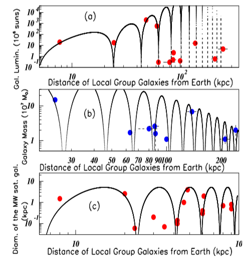
Figure 3 ThreeColor on line. Inserts (A), (B), and (C) show the Galaxy Luminosities, the Galaxy Masses and the Milky Way’s (MW) satellite galaxy (sat. gal.) diameters versus the distance of the Local Group galaxies from Earth.

Fig.	α	β	P
1	3 l.y.	0.001 l.y.⁻¹	1351 l.y.
2(a)	8 a.m.	0	0.628 kly
2(b)	8 a.m.	0	0.628 kly
2(c)	0.041 a.m.	0.5 kly⁻¹	0.628 kly
3(a)	20 10⁶ s.l.	0.09 kpc⁻¹	19.5 kpc
3(b)	40 10⁷ s.m.	-0.015 kpc	19.2 kpc
3(c)	2.6 kpc	0	17.6 kpc
4(a)	7 a.m.	0	7.85 10⁷ M0
4(b)	500 kpc	0	7.98 10⁷M0
4(c)	700 kpc	0	4.40 10⁷ M0
5	0.00126	0.0315 Mpc⁻¹	1.885 Mpc
6(a)	0.15 10¹⁴kg	0.50 years⁻¹	0.406 years
6(b)	2.75 km	0	0.402 years
7(a)	2 days	0.2 sm⁻¹	1.26 s.m.
7(b)	1000 l.y.	0.5 sm⁻¹	1.43 s.m.
8(a)	25 s.m.	-0.16 kpc⁻¹	1.51 kpc
8(b)	300 hr	-0.3 kpc⁻¹	1.35 kpc
9(a)	0.03 s.m.	2.1 s.m.⁻¹	0.346 s.m.
9(b)	5.25 l.y.	0	0.314 s.m.
9(c)	8.5 a.m.	-0.0019 s.m.⁻¹	0.427 s.m.
9(d)	385 par	0	0.427 s.m.
9(e)	3 l.y.	-0.18 l.y.⁻¹	1.88 l.y.
9(f)	8.5 a.m.	0	1.98 l.y.
10(b)	5000 Myr	0	7.54 p.c.
11	8 e.m.	0.03 e.m.⁻¹	16.3 e.m.
12(a)	1500 e.m.	-1.2 cm²/g	0.955 g/cm²
12(b)	2000 e.m.	-1.55⁽⁰⁾⁻¹	0.955⁽⁰⁾
12(c)	4000 e.m.	-0.3 hr⁻¹	4.40 hr
12(d)	0.5 e.m.	0	1.57 year
13(a)	4000 e.m.	-0.215 s/km	19.9 km/s
13(b)	10 e.m.	59 o.e.⁻¹	0.0126 o.e.

Table 1 Parameters used for the ﬁts obtained using the relation (2). The shortened units are deﬁned in the text

In the Figure 3A and Figure 3B, all data lie well on the ﬁtted curves, but in Figure 3C, two data over ﬁfteen lie notably outside the ﬁt. The three inserts (a), (b), and (c) allow to tentatively predict possible unobserved galaxies. For example the ﬁt predicts a minimum in the Galaxy luminosity at $\approx 44$ kpc from Earth, allowing for a possible missing Galaxy observation: its mass should be $\approx 10^{7}$ sun mass with a diameter $\approx 1.5$ sat. gal. Figure 4 shows the variation of diﬀerent galaxy properties¹² versus the galaxy masses (in 10⁷ sun mass units (M_⁰). These properties are the Apparent Magnitudes, the Distances of Local Group Galaxies from Earth (in kpc), and the Galaxy Distances from the Local Group Center of mass (in kpc). The ﬁt in insert (a) is not precise. The masses without error bars correspond to data given without such information and not to very precise data. Neighboring periods are observed in inserts (a) and (b), but not in insert (c) (Table 2). This last period being of the order of half the two other periods.Figure 5 shows the Galaxy group Redshifts (z)¹⁴ versus their Distance from Earth (in Mpc). Their Recession velocities (in km/s) are proportional to the redshifts, by a factor 0.0000033. A better ﬁt is observed for the seven ﬁrst data than the last three data.

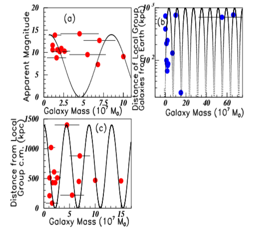
Figure 4 Color on line. Inserts (A), (B), and (C) show the Galaxy Apparent Magnitudes, the Distance of Local Group Galaxies from Earth, and the Galaxy Distances from Local Group center of mass in inserts (A), (B), and (C) respectively, versus the Galaxy masses.

Figure 5 Color on line. Redshift (z) of Galaxy groups versus their distance from Earth.

Comets

A very large number of comets are listed in Tables. Here again the gap between diﬀerent tables may be often as large as 20%, and sometimes even much larger. I selected from,¹⁵ among the ﬁrst reported data concerning comets, those having known radius. Figure 6 shows in inserts (a) and (b) the comet masses (in 10¹⁴ kg) derived from non-gravitational forces and the comet radii (in km), plotted versus the comet orbital periods (in years). Figure 6C shows the Comet Eccentricities¹⁶ versus the corresponding orbital periods (in years). The ﬁt in insert (c) is obtained using the relation (2) with $α_{0} = 0 .5, α_{1} = 0 .3,$ and P=1.82 years. Whereas both periods obtained in Figure 6A and Figure 6B are nearly the same, this near equality is not observed in Figure 6C.

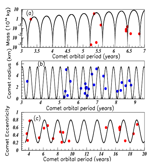
Figure 6 Color on line. Inserts (A), (B), and (C) show the Comet masses, the Comet radii, and the Comet Eccentricities versus the corresponding periods.

Black holes

The list of nearest black holes, relatively to the Solar System (within our Milky Way galaxy) are obtained in¹⁷ and¹⁸. Here again, the tables from both references list somewhat diﬀerent values, (either in l.y. or in kpc). Although a large number of black holes is reported, the list of the quoted references, corresponding to the nearest black holes, include 18 systems. However some data corresponding either to the mass or to the orbital period are missing. Figure 7A shows the black hole orbital periods (in days) versus the black hole masses (in solar mass units).^17,18 Full red marks correspond to the component A, full blue squares correspond to the component B (i.e. the A companion) of the same system. For example, the mass of the System A0620-00 (A), located at 3500 l.y. from earth, is $11 .0 \pm 2$ solar mass, and the mass of the B component of the same system is $2.7 \pm 0.1$ solar mass. Figure 7B shows the Black Hole distances from Earth (in l.y.), versus the corresponding masses (in solar masses). A masses are plotted with red full circles, B masses with blue full squares. Considering the imprecisions on data, the ﬁts describe well the data. Figure 8A shows the Black hole masses (in Sun mass units) versus their distances from Earth (in kpc).¹⁹ This Figure corresponds to Figure 7B in diﬀerent units, after reversion of coordinates. Red and blue data show the masses and their companion masses. Figure 8B shows the Binary system orbit in hours (hr) versus the corresponding distances from Earth (in kpc).

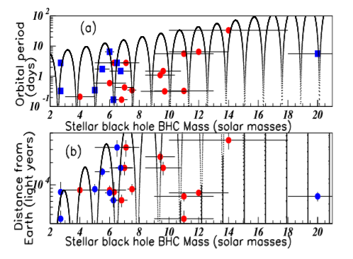
Figure 7 Color on line. Inserts (A) and (B) show Black hole masses and Binary Star System orbits versus the corresponding Black Hole distances from Earth.

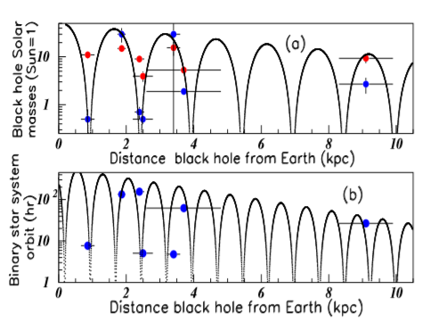
Figure 8 Color on line. Inserts (a) (and (b)) show versus the distances from Earth, the masses (and the binary system orbits.).

Stars

Several studies concerning the application of the oscillation symmetry to the stars closest to the sun are shown in Figure 9. The Figure exhibits the oscillations of several star properties plotted versus other star properties. Data corresponding to stars located at less than 16.3 l.y. from the sun²⁰ are selected. This is worth noting that for all properties, studied in Figure 9, data are not always present. This explains the variation of the number of data in the diﬀerent inserts. Figure 9A shows the diﬀerences of adjacent star masses, versus their corresponding mean values, both in sun masses (s.m.). Figure 9B shows the Star distances from Sun (in l.y.) versus the Star masses (in s.m.). Figure 9C shows the Star absolute magnitudes versus the Star masses (in s.m.). Figure 9D shows the Star parallaxes (par) versus the Star masses (in s.m.). Figure 9E shows the diﬀerences of close star distances in (l.y.) plotted versus the corresponding mean adjacent distances in (l.y.).²⁰ Insert (e) shows therefore the star distances Figure (in l.y.) like the Figure shown in insert (a) for masses. Figure 9F shows the stars absolute magnitudes (ab.m.) versus the corresponding distances from Sun (l.y.). The data on the ﬁrst ﬁve inserts are well ﬁtted. This is not the case for the data shown in the last insert.

Figure 9 Color on line. Inserts (A) shows the star mass differences versus the corresponding mean mass values. Insert (B) shows the star distances from Sun versus the star masses. Insert (C) ((D)) show the star absolute magnitudes (the star parallax) versus the star masses. Insert (E) shows the diﬀerent close star distances from Sun versus the corresponding mean distances. Insert (F) shows the stars absolute magnitudes versus the corresponding distances from Sun.

Supernovae

The table in²¹ lists 30 Supernovae with known Apparent magnitudes (a.m.) and Distances from Sun. These distances vary from 8200 up to 5.09*10⁸ l.y. Such a large range cannot be proﬁtably ﬁtted, even when using log scale. Therefore Figure 10A shows these data for only the ﬁrst nine Supernovae. The next one in the table, the Supernova SN 1885A, located in the Andromeda Galaxy, is at 2.4*10⁶ l.y. from Sun. The negative Apparent magnitude necessitates to perform the ﬁt by using the equivalent to the previously used formula (3) with again three ﬁtted parameters. These parameters are not included in Table 1 since they are diﬀerent from those of relation (2). Here $α_{0} = - 1 a .m ., α_{0} = 7 a .m .,$ and P= 4.27 .10³ l.y.

Pulsars

The table reported in²² lists eleven pulsars at distances between 156 and 300 pc and the corresponding Ages ranging between 0.0113 Myr and 7580 Myr. Figure 10B shows the Pulsar Ages (in Myr) versus their Distances to the Sun (in pc). The ﬁt is obtained using relation (2) with two parameters $α = 5000 Myr$ and P=7.54 pc $(β = 0) .$

Figure 10 Color on line. Figure 9A shows for the ﬁrst nine supernovae, the Apparent Magnitudes versus the Distances from the Sun. Insert (B) shows the Pulsar Ages versus the corresponding distances to the Sun.

How do the properties of the solar planets after introduction of two additional possible solar planet masses behave?

A few astrophysical properties concerning solar planets, studied with the discussed method, were already shown: - the Saturne, Jupiter, Uranus, and Neptune moon diameters were plotted versus the moon distances from planets,¹ - the Saturne, Uranus, and Neptune ring widths were plotted versus the planet ring radii.¹In the present paper, the possible existence oftwo new solar planets is studied. They are shown below using the improved new formula (2) to ﬁt the data. Figure 11A shows the mass spectra of the known solar planet masses.²³The diﬀerence between successive masses is plotted versus their corresponding mean values. The Jupiter mass, being very large when compared to the other planet masses is ignored. The data are well ﬁtted with the period P=16.3 e.m. The existence of two new solar planets was proposed in order to explain the strange behavior of some bodies belonging to the Kuiper’s belt.⁶ Their masses might be $\approx 0.5 e .m .$ and $\approx 10 e .m .$ respectively.⁵ The same data and ﬁt shown in Figure 11A, are reported in Figure 11B with a log x scale in order to enhance the low mass region.

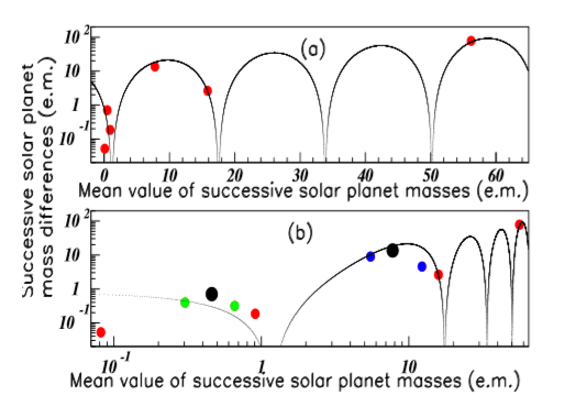
Figure 11 Color on line. Successive solar planet mass differences versus their corresponding mean values. Inserts (A) ((B)) show the data without (with) the two new possible solar planet masses. The ﬁt is the same in both inserts.

The introduction in Figure 11B of the ninth planet mass, gives rise to two new data (blue on line) and the black data between both is removed. The introduction of the tenth planet mass gives rise to two new data (green on line) and the black data between both is again removed. These two black data in insert (b) were red in insert (a). We observe that these new blue and green data are well ﬁtted with the other well-known solar planet masses. Such agreement is in favor of their existence. Several low value properties of these putative new solar planets, are predicted from Figure 12 and Figure 13, by intersection of their mass lines with the oscillations obtained using the classical solar planet properties. Figure 12 shows the Solar planet masses (in earth units) versus (a) the corresponding planet densities (in g/cm3), (b) the corresponding Plan tilting (in degrees), (c) the corresponding rotation duration (in hours), and (d) the revolution periods (in years). The diﬀerent inserts in Figure 13 show the Solar planet masses (in earth units) versus the corresponding Mean orbital speed (in km/s) (a), the corresponding Equatorial diameters (in e.u.) (b) and (d), and the corresponding Orbital eccentricities (c). The predicted values are reported in Tables 2 and 3. Larger values are of course possible occurring from oscillation pursuits.

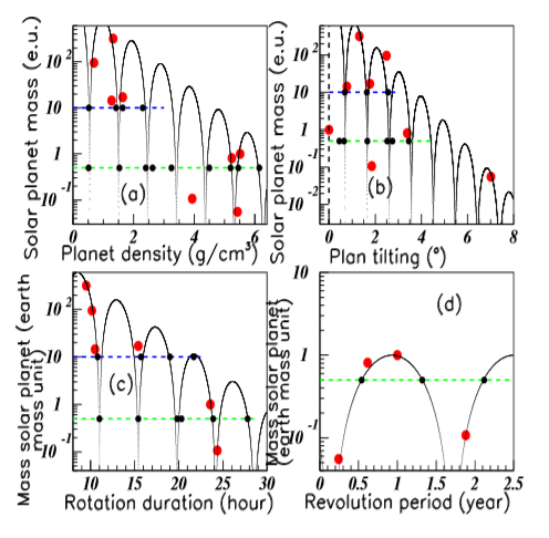
Figure 12 Color on line. Solar planet masses versus the planet densities, the plan tiltings, the rotation durations, and the revolution periods, respectively in insert (A), (B), (C), and (D).

Figure 13 Color on line. Solar planet masses versus the Mean orbital speed (in km/s) in insert (A), versus the corresponding Equatorial Diameters in insert (B) and (D), and versus the corresponding Orbital eccentricities in insert (C).

Planet	density (g/cm3)		plan tilting (o)		rotation duration(hour)		revolution period(year)
9 (blue)	0.52	1.44	0.68	1.63	11.1	15.4	-
	1.61	2.45	2.58	3.3	19	21.7	-
10 (green)	0.53	1.51	0.67	1.66	11.1	15.4	0.54	1.32
	2.45	3.41	2.6	3.53	19.8	23.75	2.12
	4.4	5.2			24.6	27.8

Table 2 Suggested properties (from Figure 12) of the anticipated ninth and tenth possible solar planets

Planet	Orbital speed (km/s)		Orbital eccentricity
9 (blue)	6.2	23.2	0.008	0.0163
			0.0435	0.056
10 (green)	5.8	25	0.0055	0.0185
	26.8	41.4	0.0435	0.056

Table 3 Suggested properties (from Figure 13) of the anticipated ninth and tenth possible solar planets

Conclusion

The oscillation symmetry method is applied to several astrophysical properties. A good agreement is often observed between data and ﬁts obtained with two or three parameters. In a few cases, we observe some data outside the ﬁt, like in Figure 2C and Figure 9F. In such cases, the ﬁrst data are well ﬁtted, but such agreement is no more observed later. The largest possible periods have been kept. Smaller periods are always possible. There is no theory which justify to use a such simple function. There is neither any argument except for masses. The ﬁts will be stabilized in the future with the increase of the number of data. However it is noteworthy that the found periods are, in most cases, rather near for oscillations corresponding to the same variable of the same bodies (Table 1). This is observed for all inserts of Figures 2–7, and Figure 8. This is also observed for only the two ﬁrst inserts of Figure 4. The nine inserts from Figure 9 are ﬁtted with three periods: $P \approx 0 .33 s .m .,$ P=0.427 s.m., and $P \approx 1.9 3 l .y .$

The oscillation symmetry method allows to predict possible unknown properties. This was performed, as an example, in the text corresponding to Figure 3, for a putative not yet observed galaxy. The controversial existence of two unobserved new solar planets is strengthened. We observe a good continuity between old data corresponding to the seven”classical” solar planets and new data. Indeed the oscillation symmetry approach shows that the predicted masses agree with the masses of the known solar planets. The method allows to predict possible values of several properties for these two unobserved planets. Even when this oscillatory behavior is clearly observed, it remains to ﬁnd the physical law which connect the properties of apparently independent bodies. For example, every solar planet mass is submitted to opposite interactions, but we do not know the relation interconnecting the diﬀerent masses. It was already emphasized that such symmetry should be often observed in nature, when opposite forces are applied. Therefore it should be observed every time when a body results from smaller substructures. In the present paper, such property is observed, although it corresponds to several bodies apparently independent.