Submit manuscript...
eISSN: 2574-9927

Material Science & Engineering International Journal

Research Article Volume 5 Issue 2

Prediction of environmental safety dynamics and management for effective functioning of the natural technical system

Bosikov Igor Ivanovich,1 Klyuev Roman Vladimirovich2

1Department of Applied Geology, North Caucasian Institute of Mining and Metallurgy (State Technological University), Russia
2Department of Industrial Power Supply, North Caucasian Institute of Mining and Metallurgy (State Technological University), Russia

Correspondence: Igor Bosikov, Department of Applied Geology, North Caucasian Institute of Mining and Metallurgy (State Technological University), 362021, North Ossetia-Alania, Vladikavkaz, Nikolayeva str. 44, Russia, Tel +7928 685 7117

Received: July 29, 2018 | Published: March 26, 2021

Citation: vanovich BI, Vladimirovich KR. Prediction of environmental safety dynamics and management for effective functioning of the natural-technical system. Material Sci & Eng. 2021;5(2):40-42. DOI: 10.15406/mseij.2021.05.00154

Download PDF

Abstract

Background: Relevance of research. The mathematical model of a singularly perturbed system with a heterogeneous morphology of the underlying surface (hilly terrain overgrown with shrubs) is considered in the article. The distribution nature of the harmful substances in this ecosystem under these infringing factors is determined. Studies using mathematical modeling and system analysis are relevant at the present stage of development and environmental safety of society.

Keywords: natural-technical system, mathematical modeling, safety, system analysis, complex estimation, diffusion equations, mining-processing complex.

Introduction

The global objectives of modeling are the issues of studying the nature of systems, the possibilities for their structural development and predicting behavior. Development and implementation of methods for predicting the dynamics and management of environmental safety of the natural-technical system is an urgent scientific task.1-2 The expediency of the studies is unquestionable, their results enable rational planning of the economic development of the region, ensure the effective investment of public funds in environmental activities and serve as a basis for environmental monitoring.2-3 In the theory of modeling the main problems are: the development of universal approaches to the construction of models, the accuracy of the simulation of the movement of their coordinates, the estimation of error values, the adequacy of the results obtained, the identification of the systems studied, the synthesis of technical devices and hypotheses.1–6 The purpose of the research: forecasting the dynamics and management of environmental safety in mountainous areas. Objects of research: natural-technical system.

Methods

The research used generalization and system analysis of experience, theoretical research, physical and mathematical modeling, laboratory and production experiment, critical understanding of research results using methods of mathematical statistics and graphic interpretation of the results of ecological and geochemical surveys with analysis of the distribution of heavy metals over the area and identification of foci chemical pollution of soils by industrial effluents.

Results

Researches of mountainous relief, overgrown with forest have been carried out. Conventionally, this relief is displayed as follows, Figure 1. Having a set of functions, they can be used to depict a mountainous relief with a more complex structure of underlying surfaces, thereby describing the spread of harmful substances in real conditions. The form of the functions y (x) was determined by mathematical experiments using the MATCAD17 environment. Studies and experiments were conducted to determine the concentration of harmful substances in ecosystems with various underlying surfaces. Solutions of equation (1) are determined.

u(x,y,ξ,t)= C 1 u 1 (x) u 1 (ξ)+ C 2 u 2 (2x) u 2 (2ξ).... MathType@MTEF@5@5@+= feaagKart1ev2aaatCvAUfeBSjuyZL2yd9gzLbvyNv2CaerbuLwBLn hiov2DGi1BTfMBaeXatLxBI9gBaerbd9wDYLwzYbItLDharqqtubsr 4rNCHbGeaGqiVu0Je9sqqrpepC0xbbL8F4rqqrFfpeea0xe9Lq=Jc9 vqaqpepm0xbba9pwe9Q8fs0=yqaqpepae9pg0FirpepeKkFr0xfr=x fr=xb9adbaqaaeGaciGaaiaabeqaamaabaabaaGcbaqcfaOaamyDai aacIcacaWG4bGaaiilaiaadMhacaGGSaGaeqOVdGNaaiilaiaadsha caGGPaGaeyypa0Jaam4qamaaBaaabaqcLbmacaaIXaaajuaGbeaaca WG1bWcdaWgaaqcfayaaKqzadGaaGymaaqcfayabaGaaiikaiaadIha caGGPaGaamyDaSWaaSbaaKqbagaajugWaiaaigdaaKqbagqaaiaacI cacqaH+oaEcaGGPaGaey4kaSIaam4qamaaBaaabaqcLbmacaaIYaaa juaGbeaacaWG1bWcdaWgaaqcfayaaKqzadGaaGOmaaqcfayabaGaai ikaiaaikdacaWG4bGaaiykaiaadwhadaWgaaqaaKqzadGaaGOmaaqc fayabaGaaiikaiaaikdacqaH+oaEcaGGPaGaaiOlaiaac6cacaGGUa GaaiOlaaaa@6780@ (1)

Figure 1 Display of mountain relief covered with forest.

Studies of the mountain relief, overgrown with forest, were carried out. Conditionally, this relief was displayed as follows (Figure 1). Having a set of functions y ( x ) : u 1 , u 2 , .. u n MathType@MTEF@5@5@+= feaagKart1ev2aaatCvAUfeBSjuyZL2yd9gzLbvyNv2CaerbuLwBLn hiov2DGi1BTfMBaeXatLxBI9gBaerbd9wDYLwzYbItLDharqqtubsr 4rNCHbGeaGqiVu0Je9sqqrpepC0xbbL8F4rqqrFfpeea0xe9Lq=Jc9 vqaqpepm0xbba9pwe9Q8fs0=yqaqpepae9pg0FirpepeKkFr0xfr=x fr=xb9adbaqaaeGaciGaaiaabeqaamaabaabaaGcbiqaaqnbjuaGca WG5bGaaiikaiaadIhacaGGPaGaaiOoaiaadwhalmaaBaaajuaGbaqc LbmacaaIXaaajuaGbeaacaGGSaGaamyDamaaBaaabaqcLbmacaaIYa aajuaGbeaacaGGSaGaaiOlaiaac6cacaWG1bWaaSbaaeaajugWaiaa d6gaaKqbagqaaaaa@49BD@  with their help, one can depict a mountain relief with a more complex structure of underlying surfaces, thereby describing the distribution of harmful substances in real conditions. The form of the functions y(x) was determined by mathematical experiments using the MATCAD17 environment.610

y(x)= u 1 (x)= π 2 4 π [ (cos(x)+ 1 9 cos(3| x |x)+ 1 25 cos(10x) ] MathType@MTEF@5@5@+= feaagKart1ev2aaatCvAUfeBSjuyZL2yd9gzLbvyNv2CaerbuLwBLn hiov2DGi1BTfMBaeXatLxBI9gBaerbd9wDYLwzYbItLDharqqtubsr 4rNCHbGeaGqiVu0Je9sqqrpepC0xbbL8F4rqqrFfpeea0xe9Lq=Jc9 vqaqpepm0xbba9pwe9Q8fs0=yqaqpepae9pg0FirpepeKkFr0xfr=x fr=xb9adbaqaaeGaciGaaiaabeqaamaabaabaaGcbaqcfaOaamyEai aacIcacaWG4bGaaiykaiabg2da9iaadwhalmaaBaaajuaGbaqcLbma caaIXaaajuaGbeaacaGGOaGaamiEaiaacMcacqGH9aqpdaWcaaqaai abec8aWbqaaiaaikdaaaGaeyOeI0YaaSaaaeaacaaI0aaabaGaeqiW dahaamaadmaabaGaaiikaiGacogacaGGVbGaai4CaiaacIcacaWG4b GaaiykaiabgUcaRmaalaaabaGaaGymaaqaaiaaiMdaaaGaci4yaiaa c+gacaGGZbGaaiikaiaaiodadaabdaqaaiaadIhaaiaawEa7caGLiW oacaWG4bGaaiykaiabgUcaRmaalaaabaGaaGymaaqaaiaaikdacaaI 1aaaaiGacogacaGGVbGaai4CaiaacIcacaaIXaGaaGimaiaadIhaca GGPaaacaGLBbGaayzxaaaaaa@6668@ (2)

y(x):= π 2 4 π [ (cos(x+5))1sin(x)+ 1 9 cos(3| x+5 |x)+ 1 25 cos[ 10(x+5) ] ] MathType@MTEF@5@5@+= feaagKart1ev2aaatCvAUfeBSjuyZL2yd9gzLbvyNv2CaerbuLwBLn hiov2DGi1BTfMBaeXatLxBI9gBaerbd9wDYLwzYbItLDharqqtubsr 4rNCHbGeaGqiVu0Je9sqqrpepC0xbbL8F4rqqrFfpeea0xe9Lq=Jc9 vqaqpepm0xbba9pwe9Q8fs0=yqaqpepae9pg0FirpepeKkFr0xfr=x fr=xb9adbaqaaeGaciGaaiaabeqaamaabaabaaGcbaqcfaOaamyEai aacIcacaWG4bGaaiykaiaacQdacqGH9aqpdaWcaaqaaiabec8aWbqa aiaaikdaaaGaeyOeI0YaaSaaaeaacaaI0aaabaGaeqiWdahaamaadm aabaGaaiikaiGacogacaGGVbGaai4CaiaacIcacaWG4bGaey4kaSIa aGynaiaacMcacaGGPaGaeyOeI0IaaGymaiGacohacaGGPbGaaiOBai aacIcacaWG4bGaaiykaiabgUcaRmaalaaabaGaaGymaaqaaiaaiMda aaGaci4yaiaac+gacaGGZbGaaiikaiaaiodadaabdaqaaiaadIhacq GHRaWkcaaI1aaacaGLhWUaayjcSdGaeyyXICTaamiEaiaacMcacqGH RaWkdaWcaaqaaiaaigdaaeaacaaIYaGaaGynaaaaciGGJbGaai4Bai aacohadaWadaqaaiaaigdacaaIWaGaaiikaiaadIhacqGHRaWkcaaI 1aGaaiykaaGaay5waiaaw2faaaGaay5waiaaw2faaaaa@7041@ (3)

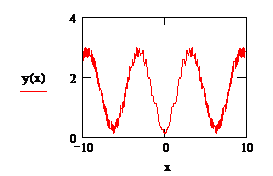
Figure 2 & Figure 3, here y(x): u 1 , u 2 ,.. MathType@MTEF@5@5@+= feaagKart1ev2aaatCvAUfeBSjuyZL2yd9gzLbvyNv2CaerbuLwBLn hiov2DGi1BTfMBaeXatLxBI9gBaerbd9wDYLwzYbItLDharqqtubsr 4rNCHbGeaGqiVu0Je9sqqrpepC0xbbL8F4rqqrFfpeea0xe9Lq=Jc9 vqaqpepm0xbba9pwe9Q8fs0=yqaqpepae9pg0FirpepeKkFr0xfr=x fr=xb9adbaqaaeGaciGaaiaabeqaamaabaabaaGcbaqcfaOaamyEai aacIcacaWG4bGaaiykaiaacQdacaWG1bWaaSbaaeaajugWaiaaigda aKqbagqaaiaacYcacaWG1bWaaSbaaeaajugWaiaaikdaaKqbagqaai aacYcacaGGUaGaaiOlaaaa@447F@

Figure 2 The display of a hilly relief covered with shrubs.

Figure 3 Display a hilly relief covered with grass.

y(x):= π 2 2 π [ (cos(x))1sin(| x |)+ 1 9 cos(3| x9 |x)+ 1 25 cos(10x)) ] MathType@MTEF@5@5@+= feaagKart1ev2aaatCvAUfeBSjuyZL2yd9gzLbvyNv2CaerbuLwBLn hiov2DGi1BTfMBaeXatLxBI9gBaerbd9wDYLwzYbItLDharqqtubsr 4rNCHbGeaGqiVu0Je9sqqrpepC0xbbL8F4rqqrFfpeea0xe9Lq=Jc9 vqaqpepm0xbba9pwe9Q8fs0=yqaqpepae9pg0FirpepeKkFr0xfr=x fr=xb9adbaqaaeGaciGaaiaabeqaamaabaabaaGcbaqcfaOaamyEai aacIcacaWG4bGaaiykaiaacQdacqGH9aqpdaWcaaqaaiabec8aWbqa aiaaikdaaaGaeyOeI0YaaSaaaeaacaaIYaaabaGaeqiWdahaamaadm aabaGaaiikaiGacogacaGGVbGaai4CaiaacIcacaWG4bGaaiykaiaa cMcacqGHsislcaaIXaGaci4CaiaacMgacaGGUbGaaiikamaaemaaba GaamiEaaGaay5bSlaawIa7aiaacMcacqGHRaWkdaWcaaqaaiaaigda aeaacaaI5aaaaiGacogacaGGVbGaai4CaiaacIcacaaIZaWaaqWaae aacaWG4bGaeyOeI0IaaGyoaaGaay5bSlaawIa7aiabgwSixlaadIha caGGPaGaey4kaSYaaSaaaeaacaaIXaaabaGaaGOmaiaaiwdaaaGaci 4yaiaac+gacaGGZbGaaiikaiaaigdacaaIWaGaamiEaiaacMcacaGG PaaacaGLBbGaayzxaaaaaa@6EE9@ (4)

In the course of the studies, the distribution of harmful substances in the hilly terrain overgrown with shrubs was determined. To do this, initially effective coefficients were found.614

u ¯ 1 = 0 10 0 1 y 1 (x) y 1 (ξ)dxdξ= 20.741 MathType@MTEF@5@5@+= feaagKart1ev2aaatCvAUfeBSjuyZL2yd9gzLbvyNv2CaerbuLwBLn hiov2DGi1BTfMBaeXatLxBI9gBaerbd9wDYLwzYbItLDharqqtubsr 4rNCHbGeaGqiVu0Je9sqqrpepC0xbbL8F4rqqrFfpeea0xe9Lq=Jc9 vqaqpepm0xbba9pwe9Q8fs0=yqaqpepae9pg0FirpepeKkFr0xfr=x fr=xb9adbaqaaeGaciGaaiaabeqaamaabaabaaGcbaqcfaOabmyDay aaraWcdaWgaaqcfayaaKqzadGaaGymaaqcfayabaGaeyypa0Zaa8qC aeaadaWdXbqaaiaadMhadaWgaaqaaiaaigdaaeqaaiaacIcacaWG4b GaaiykaiaadMhadaWgaaqaaiaaigdaaeqaaiaacIcacqaH+oaEcaGG PaGaamizaiaadIhacaWGKbGaeqOVdGNaeyypa0dabaqcLbmacaaIWa aajuaGbaqcLbmacaaIXaaajuaGcqGHRiI8aaqaaKqzadGaaGimaaqc fayaaKqzadGaaGymaiaaicdaaKqbakabgUIiYdGaaGOmaiaaicdaca GGUaGaaG4naiaaisdacaaIXaaaaa@5E23@ , u ¯ 2 = 0 10 0 1 y 2 (x) y 2 (ξ)dxdξ= 22.458 MathType@MTEF@5@5@+= feaagKart1ev2aaatCvAUfeBSjuyZL2yd9gzLbvyNv2CaerbuLwBLn hiov2DGi1BTfMBaeXatLxBI9gBaerbd9wDYLwzYbItLDharqqtubsr 4rNCHbGeaGqiVu0Je9sqqrpepC0xbbL8F4rqqrFfpeea0xe9Lq=Jc9 vqaqpepm0xbba9pwe9Q8fs0=yqaqpepae9pg0FirpepeKkFr0xfr=x fr=xb9adbaqaaeGaciGaaiaabeqaamaabaabaaGcbaqcfaOabmyDay aaraWaaSbaaeaajugWaiaaikdaaKqbagqaaiabg2da9maapehabaWa a8qCaeaacaWG5bWaaSbaaeaajugWaiaaikdaaKqbagqaaiaacIcaca WG4bGaaiykaiaadMhadaWgaaqaaKqzadGaaGOmaaqcfayabaGaaiik aiabe67a4jaacMcacaWGKbGaamiEaiaadsgacqaH+oaEcqGH9aqpae aajugWaiaaicdaaKqbagaajugWaiaaigdaaKqbakabgUIiYdaabaqc LbmacaaIWaaajuaGbaqcLbmacaaIXaGaaGimaaqcfaOaey4kIipaca aIYaGaaGOmaiaac6cacaaI0aGaaGynaiaaiIdaaaa@610C@

y 1 (x)=π 1 2 4 π [ cos(x+5)sin(x)+ 1 9 cos(3| x+5 |)x+ 1 25 cos10(x+5) ] MathType@MTEF@5@5@+= feaagKart1ev2aaatCvAUfeBSjuyZL2yd9gzLbvyNv2CaerbuLwBLn hiov2DGi1BTfMBaeXatLxBI9gBaerbd9wDYLwzYbItLDharqqtubsr 4rNCHbGeaGqiVu0Je9sqqrpepC0xbbL8F4rqqrFfpeea0xe9Lq=Jc9 vqaqpepm0xbba9pwe9Q8fs0=yqaqpepae9pg0FirpepeKkFr0xfr=x fr=xb9adbaqaaeGaciGaaiaabeqaamaabaabaaGcbaqcfaOaamyEam aaBaaabaqcLbmacaaIXaaajuaGbeaacaGGOaGaamiEaiaacMcacqGH 9aqpcqaHapaCdaWcaaqaaiaaigdaaeaacaaIYaaaaiabgkHiTmaala aabaGaaGinaaqaaiabec8aWbaadaWadaqaaiGacogacaGGVbGaai4C aiaacIcacaWG4bGaey4kaSIaaGynaiaacMcacqGHsislciGGZbGaai yAaiaac6gacaGGOaGaamiEaiaacMcacqGHRaWkdaWcaaqaaiaaigda aeaacaaI5aaaaiGacogacaGGVbGaai4CaiaacIcacaaIZaWaaqWaae aacaWG4bGaey4kaSIaaGynaaGaay5bSlaawIa7aiaacMcacaWG4bGa ey4kaSYaaSaaaeaacaaIXaaabaGaaGOmaiaaiwdaaaGaci4yaiaac+ gacaGGZbGaaGymaiaaicdacaGGOaGaamiEaiabgUcaRiaaiwdacaGG PaaacaGLBbGaayzxaaaaaa@6C86@ (5)

y 2 (2x)=π 1 2 4 π [ cos2(x+5)sin2(x)+ 1 9 cos(3| 2x+5 |)2x+ 1 25 cos10(2x+5) ] MathType@MTEF@5@5@+= feaagKart1ev2aaatCvAUfeBSjuyZL2yd9gzLbvyNv2CaerbuLwBLn hiov2DGi1BTfMBaeXatLxBI9gBaerbd9wDYLwzYbItLDharqqtubsr 4rNCHbGeaGqiVu0Je9sqqrpepC0xbbL8F4rqqrFfpeea0xe9Lq=Jc9 vqaqpepm0xbba9pwe9Q8fs0=yqaqpepae9pg0FirpepeKkFr0xfr=x fr=xb9adbaqaaeGaciGaaiaabeqaamaabaabaaGcbaqcfaOaamyEam aaBaaabaqcLbmacaaIYaaajuaGbeaacaGGOaGaaGOmaiaadIhacaGG PaGaeyypa0JaeqiWda3aaSaaaeaacaaIXaaabaGaaGOmaaaacqGHsi sldaWcaaqaaiaaisdaaeaacqaHapaCaaWaamWaaeaaciGGJbGaai4B aiaacohacaaIYaGaaiikaiaadIhacqGHRaWkcaaI1aGaaiykaiabgk HiTiGacohacaGGPbGaaiOBaiaaikdacaGGOaGaamiEaiaacMcacqGH RaWkdaWcaaqaaiaaigdaaeaacaaI5aaaaiGacogacaGGVbGaai4Cai aacIcacaaIZaWaaqWaaeaacaaIYaGaamiEaiabgUcaRiaaiwdaaiaa wEa7caGLiWoacaGGPaGaaGOmaiaadIhacqGHRaWkdaWcaaqaaiaaig daaeaacaaIYaGaaGynaaaaciGGJbGaai4BaiaacohacaaIXaGaaGim aiaacIcacaaIYaGaamiEaiabgUcaRiaaiwdacaGGPaaacaGLBbGaay zxaaaaaa@70EF@ (6)

γ 1 =2.291 MathType@MTEF@5@5@+= feaagKart1ev2aaatCvAUfeBSjuyZL2yd9gzLbvyNv2CaerbuLwBLn hiov2DGi1BTfMBaeXatLxBI9gBaerbd9wDYLwzYbItLDharqqtubsr 4rNCHbGeaGqiVu0Je9sqqrpepC0xbbL8F4rqqrFfpeea0xe9Lq=Jc9 vqaqpepm0xbba9pwe9Q8fs0=yqaqpepae9pg0FirpepeKkFr0xfr=x fr=xb9adbaqaaeGaciGaaiaabeqaamaabaabaaGcbiqaaqnbjuaGcq aHZoWzlmaaBaaajuaGbaqcLbmacaaIXaaajuaGbeaacqGH9aqpcqGH sislcaaIYaGaaiOlaiaaikdacaaI5aGaaGymaaaa@41D2@ , γ 2 =2.291 MathType@MTEF@5@5@+= feaagKart1ev2aaatCvAUfeBSjuyZL2yd9gzLbvyNv2CaerbuLwBLn hiov2DGi1BTfMBaeXatLxBI9gBaerbd9wDYLwzYbItLDharqqtubsr 4rNCHbGeaGqiVu0Je9sqqrpepC0xbbL8F4rqqrFfpeea0xe9Lq=Jc9 vqaqpepm0xbba9pwe9Q8fs0=yqaqpepae9pg0FirpepeKkFr0xfr=x fr=xb9adbaqaaeGaciGaaiaabeqaamaabaabaaGcbiqaaqnbjuaGcq aHZoWzlmaaBaaajuaGbaqcLbmacaaIYaaajuaGbeaacqGH9aqpcqGH sislcaaIYaGaaiOlaiaaikdacaaI5aGaaGymaaaa@41D3@

The system for finding Ci (t)

{ μ C ˙ 1 + γ ¯ 1 u ¯ 1 C 1 cost=0 μ C ˙ 2 + γ ¯ 2 u ¯ 2 C 2 cos2t=0 ..................................... μ C ˙ n + γ ¯ n u ¯ n C n cos2t=0 MathType@MTEF@5@5@+= feaagKart1ev2aaatCvAUfeBSjuyZL2yd9gzLbvyNv2CaerbuLwBLn hiov2DGi1BTfMBaeXatLxBI9gBaerbd9wDYLwzYbItLDharqqtubsr 4rNCHbGeaGqiVu0Je9sqqrpepC0xbbL8F4rqqrFfpeea0xe9Lq=Jc9 vqaqpepm0xbba9pwe9Q8fs0=yqaqpepae9pg0FirpepeKkFr0xfr=x fr=xb9adbaqaaeGaciGaaiaabeqaamaabaabaaGcbiqaaqnbjuaGda GabaabaeqabaGaeqiVd0Mabm4qayaacaWaaSbaaeaajugWaiaaigda aKqbagqaaiabgUcaRmaalaaabaGafq4SdCMbaebadaWgaaqaaKqzad GaaGymaaqcfayabaaabaGabmyDayaaraWaaSbaaeaajugWaiaaigda aKqbagqaaaaacaWGdbWcdaWgaaqcfayaaKqzadGaaGymaaqcfayaba GaeyOeI0Iaci4yaiaac+gacaGGZbGaamiDaiabg2da9iaaicdaaeaa cqaH8oqBceWGdbGbaiaadaWgaaqaaKqzadGaaGOmaaqcfayabaGaey 4kaSYaaSaaaeaacuaHZoWzgaqeamaaBaaabaqcLbmacaaIYaaajuaG beaaaeaaceWG1bGbaebadaWgaaqaaKqzadGaaGOmaaqcfayabaaaai aadoeadaWgaaqaaKqzadGaaGOmaaqcfayabaGaeyOeI0Iaci4yaiaa c+gacaGGZbGaaGOmaiaadshacqGH9aqpcaaIWaaabaGaaiOlaiaac6 cacaGGUaGaaiOlaiaac6cacaGGUaGaaiOlaiaac6cacaGGUaGaaiOl aiaac6cacaGGUaGaaiOlaiaac6cacaGGUaGaaiOlaiaac6cacaGGUa GaaiOlaiaac6cacaGGUaGaaiOlaiaac6cacaGGUaGaaiOlaiaac6ca caGGUaGaaiOlaiaac6cacaGGUaGaaiOlaiaac6cacaGGUaGaaiOlai aac6cacaGGUaGaaiOlaaqaaiabeY7aTjqadoeagaGaamaaBaaabaqc LbmacaWGUbaajuaGbeaacqGHRaWkdaWcaaqaaiqbeo7aNzaaraWaaS baaeaajugWaiaad6gaaKqbagqaaaqaaiqadwhagaqeamaaBaaabaqc LbmacaWGUbaajuaGbeaaaaGaam4qamaaBaaabaqcLbmacaWGUbaaju aGbeaacqGHsislciGGJbGaai4BaiaacohacaaIYaGaamiDaiabg2da 9iaaicdaaaGaay5Eaaaaaa@9CF2@         (7)

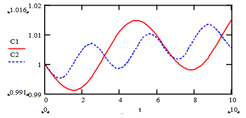
To determine the solution of the system (7), we used the program EULER , at μ=8 MathType@MTEF@5@5@+= feaagKart1ev2aaatCvAUfeBSjuyZL2yd9gzLbvyNv2CaerbuLwBLn hiov2DGi1BTfMBaeXatLxBI9gBaerbd9wDYLwzYbItLDharqqtubsr 4rNCHbGeaGqiVu0Je9sqqrpepC0xbbL8F4rqqrFfpeea0xe9Lq=Jc9 vqaqpepm0xbba9pwe9Q8fs0=yqaqpepae9pg0FirpepeKkFr0xfr=x fr=xb9adbaqaaeGaciGaaiaabeqaamaabaabaaGcbiqaaqnbjuaGcq aH8oqBcqGH9aqpcaaI4aaaaa@3ADD@ (Figure 4).

Figure 4 Charts of coefficients С1(t),С2(t).

{ μ C ˙ 1 0,11 C 1 cost=0 μ C ˙ 2 0,102 C 2 cos2t=0 MathType@MTEF@5@5@+= feaagKart1ev2aaatCvAUfeBSjuyZL2yd9gzLbvyNv2CaerbuLwBLn hiov2DGi1BTfMBaeXatLxBI9gBaerbd9wDYLwzYbItLDharqqtubsr 4rNCHbGeaGqiVu0Je9sqqrpepC0xbbL8F4rqqrFfpeea0xe9Lq=Jc9 vqaqpepm0xbba9pwe9Q8fs0=yqaqpepae9pg0FirpepeKkFr0xfr=x fr=xb9adbaqaaeGaciGaaiaabeqaamaabaabaaGcbiqaaqnbjuaGda GabaabaeqabaGaeqiVd0Mabm4qayaacaWaaSbaaeaajugWaiaaigda aKqbagqaaiabgkHiTiaaicdacaGGSaGaaGymaiaaigdacaWGdbWcda WgaaqcfayaaKqzadGaaGymaaqcfayabaGaeyOeI0Iaci4yaiaac+ga caGGZbGaamiDaiabg2da9iaaicdaaeaacqaH8oqBceWGdbGbaiaada WgaaqaaKqzadGaaGOmaaqcfayabaGaeyOeI0IaaGimaiaacYcacaaI XaGaaGimaiaaikdacaWGdbWaaSbaaeaajugWaiaaikdaaKqbagqaai abgkHiTiGacogacaGGVbGaai4CaiaaikdacaWG0bGaeyypa0JaaGim aaaacaGL7baaaaa@601C@ (8)

During the active experiment, a function was obtained that determines the nature of the change in harmful substances in the atmosphere with a hilly surface overgrown with shrubs.10–21

u(x,y,ξ,t)= C 1 u 1 (x) u 1 (ξ)+ C 2 u 2 (2x) u 2 (2ξ)....+ C n u n (2x) u n (2ξ) MathType@MTEF@5@5@+= feaagKart1ev2aaatCvAUfeBSjuyZL2yd9gzLbvyNv2CaerbuLwBLn hiov2DGi1BTfMBaeXatLxBI9gBaerbd9wDYLwzYbItLDharqqtubsr 4rNCHbGeaGqiVu0Je9sqqrpepC0xbbL8F4rqqrFfpeea0xe9Lq=Jc9 vqaqpepm0xbba9pwe9Q8fs0=yqaqpepae9pg0FirpepeKkFr0xfr=x fr=xb9adbaqaaeGaciGaaiaabeqaamaabaabaaGcbiqaaqnbjuaGca WG1bGaaiikaiaadIhacaGGSaGaamyEaiaacYcacqaH+oaEcaGGSaGa amiDaiaacMcacqGH9aqpcaWGdbWcdaWgaaqcfayaaKqzadGaaGymaa qcfayabaGaamyDamaaBaaabaqcLbmacaaIXaaajuaGbeaacaGGOaGa amiEaiaacMcacaWG1bWaaSbaaeaacaaIXaaabeaacaGGOaGaeqOVdG NaaiykaiabgUcaRiaadoeadaWgaaqaaKqzadGaaGOmaaqcfayabaGa amyDamaaBaaabaqcLbmacaaIYaaajuaGbeaacaGGOaGaaGOmaiaadI hacaGGPaGaamyDamaaBaaabaqcLbmacaaIYaaajuaGbeaacaGGOaGa aGOmaiabe67a4jaacMcacaGGUaGaaiOlaiaac6cacaGGUaGaey4kaS Iaam4qamaaBaaabaqcLbmacaWGUbaajuaGbeaacaWG1bWaaSbaaeaa jugWaiaad6gaaKqbagqaaiaacIcacaaIYaGaamiEaiaacMcacaWG1b WaaSbaaeaajugWaiaad6gaaKqbagqaaiaacIcacaaIYaGaeqOVdGNa aiykaaaa@7865@ (9)

u 1 (x)=π 1 2 4 π [ cos(x+5)sin(x)+ 1 9 cos(3| x+5 |)x+ 1 25 cos10(x+5) ] MathType@MTEF@5@5@+= feaagKart1ev2aaatCvAUfeBSjuyZL2yd9gzLbvyNv2CaerbuLwBLn hiov2DGi1BTfMBaeXatLxBI9gBaerbd9wDYLwzYbItLDharqqtubsr 4rNCHbGeaGqiVu0Je9sqqrpepC0xbbL8F4rqqrFfpeea0xe9Lq=Jc9 vqaqpepm0xbba9pwe9Q8fs0=yqaqpepae9pg0FirpepeKkFr0xfr=x fr=xb9adbaqaaeGaciGaaiaabeqaamaabaabaaGcbiqaaqnbjuaGca WG1bWaaSbaaeaajugWaiaaigdaaKqbagqaaiaacIcacaWG4bGaaiyk aiabg2da9iabec8aWnaalaaabaGaaGymaaqaaiaaikdaaaGaeyOeI0 YaaSaaaeaacaaI0aaabaGaeqiWdahaamaadmaabaGaci4yaiaac+ga caGGZbGaaiikaiaadIhacqGHRaWkcaaI1aGaaiykaiabgkHiTiGaco hacaGGPbGaaiOBaiaacIcacaWG4bGaaiykaiabgUcaRmaalaaabaGa aGymaaqaaiaaiMdaaaGaci4yaiaac+gacaGGZbGaaiikaiaaiodada abdaqaaiaadIhacqGHRaWkcaaI1aaacaGLhWUaayjcSdGaaiykaiaa dIhacqGHRaWkdaWcaaqaaiaaigdaaeaacaaIYaGaaGynaaaaciGGJb Gaai4BaiaacohacaaIXaGaaGimaiaacIcacaWG4bGaey4kaSIaaGyn aiaacMcaaiaawUfacaGLDbaaaaa@6D5D@ (10)

u 2 (2x)=π 1 2 4 π [ cos(2x+5)sin(2x)+ 1 9 cos(3| 2x+5 |)x+ 1 25 cos10(2x+5) ] MathType@MTEF@5@5@+= feaagKart1ev2aaatCvAUfeBSjuyZL2yd9gzLbvyNv2CaerbuLwBLn hiov2DGi1BTfMBaeXatLxBI9gBaerbd9wDYLwzYbItLDharqqtubsr 4rNCHbGeaGqiVu0Je9sqqrpepC0xbbL8F4rqqrFfpeea0xe9Lq=Jc9 vqaqpepm0xbba9pwe9Q8fs0=yqaqpepae9pg0FirpepeKkFr0xfr=x fr=xb9adbaqaaeGaciGaaiaabeqaamaabaabaaGcbiqaaqnbjuaGca WG1bWaaSbaaeaajugWaiaaikdaaKqbagqaaiaacIcacaaIYaGaamiE aiaacMcacqGH9aqpcqaHapaCdaWcaaqaaiaaigdaaeaacaaIYaaaai abgkHiTmaalaaabaGaaGinaaqaaiabec8aWbaadaWadaqaaiGacoga caGGVbGaai4CaiaacIcacaaIYaGaamiEaiabgUcaRiaaiwdacaGGPa GaeyOeI0Iaci4CaiaacMgacaGGUbGaaiikaiaaikdacaWG4bGaaiyk aiabgUcaRmaalaaabaGaaGymaaqaaiaaiMdaaaGaci4yaiaac+gaca GGZbGaaiikaiaaiodadaabdaqaaiaaikdacaWG4bGaey4kaSIaaGyn aaGaay5bSlaawIa7aiaacMcacaWG4bGaey4kaSYaaSaaaeaacaaIXa aabaGaaGOmaiaaiwdaaaGaci4yaiaac+gacaGGZbGaaGymaiaaicda caGGOaGaaGOmaiaadIhacqGHRaWkcaaI1aGaaiykaaGaay5waiaaw2 faaaaa@710A@ (11)

Discussion

Mathematical models of the mountain terrain were developed to study the environmental safety of the environment. Analyzing the complex relief of the mountainous terrain, qualitative and quantitative characteristics of environmental indicators were determined. Using the information received, it is possible to assess in more detail and effectively the ecological situation in mountainous areas. Most of the studies were carried out without taking into account the flat terrain, therefore, it is necessary to develop a methodology for the analysis of environmental indicators for this locality, which goes beyond previous studies. Consequently, many issues need to be analyzed in the following studies on the environmental safety of different territories.18–21

Research results

A methodology for managing ecosystems in the mountainous region has been developed. The possibility of increasing the efficiency of ecosystem management in a mountainous region in the conditions of a natural and technical system by using the methodology for predicting the dynamics and managing environmental safety in mountainous areas has been substantiated.

Conclusion

The use of the proposed methodology and the technical means developed by the authors using the MATCAD17 environment increases the information saturation of environmental monitoring, which contributes to the solution of issues related to the effectiveness of environmental safety management and a comprehensive assessment of the state of the environment. The impact of industrial facilities on the surrounding ecosystems of the mining complex.

Funding details

Results of the study of water and energy HPP parameters were included in the plan of research and development of the technology platform "Future of Renewable Energy Technologies" (2020), in which NCIMM (STU) has been included since 2013. The results were reflected in the Grant of the President of the Russian Federation for support of young scientists: MK-2576.2009.8 on "Investigation of water-power modes, static and dynamic stability of the high-pressure power plant".

Acknowledgments

The authors are grateful to I.E. Vasiliev for the proposal to develop a methodology for predicting the dynamics and management of environmental safety in mountainous areas, N.I. Tsygulyov for helping to compile a mathematical model of a singularly perturbed system with a heterogeneous morphology of the underlying surface.

Conflicts of interest

Authors declare that there is no conflict of interest.

References

  1. Golik VI, Razorenov YI, Polukhin ON. Metal extraction from ore benefication codas by means of lixiviation in a disintegrator. International Journal of Applied Engineering Research. 2015;10(17):38105–38109.
  2. Golik V, Komashchenko V, Morkun V, et al. Metal deposits combined development experience. Metallurgical and Mining Industry. 2015;7(6):591–594.
  3. Youn RB, Klyuev RV, Bosikov II, et al. The petroleum potential estimation of the north caucasus and kazakhstan territories with the help of the structural-geodynamic prerequisites. Ustojchivoe razvitie gornyh territorij (Sustainable Development of Mountain Territories). 2017;9(2):172–178.
  4. Bosikov II, Klyuev RV. System analysis methods for natural and industrial system of mining and metallurgical complex. Vladikavkaz. A Ju Publ; 2015:124.
  5. Bosikov II, Klyuev RV. Development of methods and algorithms for increasing the efficiency of the functioning of the industrial and technical system. Vladikavkaz, Terek. 2018:237.
  6. Belov PG. System analysis and modeling of hazardous processes in the technosphere. Moscow. Publishing Center "Academy"; 2003:512.
  7. Spitsnadel VN. Theory and practice of optimal decision making. SPb: Publishing house; 2002:394.
  8. Benardos A, Athanasiadis I, Katsoulakos N. Modern earth sheltered constructions: a paradigm of green engineering. Tunnelling and Underground Space Technology. 2014;41:46–52.
  9. Banov M, Bech J, Ivanov P, et al. Resolving of environmental problems caused by the processing of copper ore. Bulgarian Journal of Agricultural Science. 2014;20(3):581–589.
  10. Sokolov IV, Smirnov AA, Antipin Yu G, et al. The Effect of recovery on the effectiveness of the technology of underground mining of ore deposits. Izv. universities. Mining journal. 2012;3:4–11.
  11. Sokolov IV, Antipin YuG. Systematization and economic-mathematical modeling of the options of opening underground reserves at the combined development of deposits. Mining magazine. 2012;1:67–71.
  12. Andreev LI, Kravchuk IL, Han KO. Directions of system development production and maintenance of mining. GORN. 2011;11:269–275.
  13. Trubetskoy KN, Kornilkov SV, Yakovlev BL. New approaches to obespecheniu sustainable development of mining. Mining journal. 2012;1:15–19.
  14. Kaplunov DR, Kalmykov VN, Ryl'nikova MV. Combined Geotechnology. Moscow: Ore and Metals. 2003:560.
  15. Zaidenvarg VE, Naviti AM, Semimobile JG. Scientific basis for integrated environmental monitoring of the area mines closed. Moscow: Rosinformugol. 2002:225.
  16. Kabirov VR, Reyshahri EI. Economic evaluation of the effectiveness of the development group of geographically contiguous deposits of metallic minerals. Internet journal. 2014;2(21):1–8.
  17. Balandin KA. Cost Function of the enterprise, taking into account the costs of managing a production capacity. International research journal. 2014;3-3(22):6–9.
  18. Moore P. Assignment autonomy. International Mining. 2015:14–24.
  19. Thrybom L, Neander J, Hansen E, et al. Future Challenges of Positioning in Underground Mines. IFAC-PapersOnLine. 2015;48(10):222–226.
  20. Cai C, Luo X, Zhu J. Modified algorithm of combined GPS/GLONASS precise point positioning for applications in open-pit mines. Transactions of Nonferrous Metals Society of China. 2014;24(5):1547–1553.
  21. Hammer F, Pichler M, Fenzl H, et al. An acoustic position estimation prototype system for underground mining safety. Applied Acoustics. 2015;92:61–74.
Creative Commons Attribution License

©2021 vanovich, et al. This is an open access article distributed under the terms of the, which permits unrestricted use, distribution, and build upon your work non-commercially.