Gene optimization is a popular problem to research both in experiment and in analyzing data. Today, there are many methods and models applied to this problem but some characteristic patterns in data which have not been learnt such as missing data. Moreover, missing data contains lack of information in parameters of differential equation so some differential equations of biological system cannot be computed. The aim of this study is to evaluate and learn from missing information in data as well as in solving differential equation. We have two different models for two problems. Adaptive Neuro-fuzzy inference system (ANFIS) dealt with missing information in data. Fuzzy differential equations (FDEs) are used to model and compute differential equation when it missed information in the equation. Overall, the results in ANFIS model are larger than 90% both in testing and in training. Besides that, the statistical testing in FDEs model has not a good performance in using to predict gene expression with data. However, we propose a new process to use fuzzy methods to solve differential equation and train data when those are missing some essential values.

Keywords: gene optimization, fuzzy differential equation, recombinant protein, adaptive neuro-fuzzy inference system, synthetic gene designer

ANFIS, adaptive neuro-fuzzy inference system; FDEs, fuzzy differential equations; SGD, synthetic gene designer; CAI, codon adaption index; GA, genetic algorithm

Once a recombinant DNA is inserted into bacteria, these bacteria will make protein based on this recombinant DNA. This protein is known as "Recombinant protein". The demand of recombinant proteins has increased as more applications in several fields become a commercial reality.¹ For instance, today, more than 75 recombinant proteins are utilized as pharmaceuticals, and more than 360 new medicines based on recombinant proteins are under development (www.phrma.org).

The performance of the protein can be strongly affected by the gene expression in the host. In biology, the researchers chose the best appropriate host, which has more efficient, and cell growth for the recombinant protein. There is a general rule for this method is that the simplest cell that can provide a functional product in a time- and cost-effective manner is the best host.² However, this approach takes a long time in choosing and is not effective for mass production. The researchers lead to gene optimization to adjust the target gene that appropriate to gene expression in the host.

Many research programs have been started with the goal of using different features in DNA sequence that influence protein expression levels to optimize gene in host cell. However, the collection of data points for those features is small and uncertain. Sometimes, it misses some important information in building model. Fuzzy methods thus are needed for using analysis and estimation uncertain and missing information.

Condon usage has most often been studied in gene optimization. In,³ Puigbo et al.,³ introduced the programs used One amino acid-one codon method in gene optimization includes OPTIMIZER, JCAT, Synthetic Gene Designer (SGD), DNA Works, etc. So far, the limitation of those programs is that if the research uses different reference set for HEG, the result of gene optimization is different. Moreover, it existed some genes with extremely low codon adaption index (CAI) values are highly expressed.⁴ As we know, one amino acid-one codon is a method that replaced less frequently codon to high frequently codon used in host cell. This approach increased CAI in gene optimization. Thus, we can miss some optimized genes that have low CAI.

Powerful mathematical methods for modeling biochemical reaction systems by means of differential equations have been developed in the past century, especially in the context of metabolic processes.^5–7 Johan proposed three differential equations as three stages (Gene activation, Transcription, and Translation) in gene expression. The model is complete in modeling from the beginning of the gene activation to the translation by using stochastic process and chemical equations. A limitation of this model is using in computation and analysis. Specifically, missing information for parameters in differential equation is a big problem in using it.

Zhang et al.,⁸ confirmed that most of biological data are derived from logically-designed, hypothesis-driven experiments, which may contain various noises, and fuzzy logic provides a way for biologists to incorporate data that might otherwise be difficult to incorporate into computer models. Woolf et al. 2000 used fuzzy inference system and fuzzy set to model transcription stage in gene expression process. In 2003 and 2004, Dembele and Vinterbo separately apply fuzzy logic to analyze and model gene expression data.^9,10 Moreover, uncertainty is an attribute of information¹¹ and the use of fuzzy differential equations (FDEs) is a natural way to model dynamic systems with embedded uncertainty.¹²

Because of these things, we hypothesize that to use adaptive neuron – fuzzy inference system to deal with biological data and to use fuzzy differential equation to make those differential equations used in computation and computer models. We then chose adaptive neuron – fuzzy inference system model as the “fitness” function into genetic algorithm (GA) for searching the best sequence that adapt gene expression process in host cell (gene optimization).

There are two models which we applied in this article to gene optimization: Adaptive Neuro – Fuzzy Inference System (ANFIS) and Fuzzy Differential Equations (FDEs). The ANFIS model was used as a learner to train biological data and predict gene expression level from features used in training. We then combined with genetic algorithm (GA) to gene optimization.

Fuzzy Differential Equation model was a process that we solve fuzzy differential equation for translation stage in gene expression based on two models: differential equation for gene activation and fuzzy inference system for transcription.

Adaptive neuro-fuzzy inference system and genetic algorithms

ANFIS used fuzzy inference system to data modeling. As we know, the shape of membership functions depends on parameters, and changing these parameters change the shape of membership function. Instead of looking at the data to choose the shape and the parameters of the membership function, we can automatically choose these parameters by training on data (www.mathworks.com).

ANFIS includes two components: fuzzy inference system and neuron network.¹³ Fuzzy inference is the process of formulating the mapping from a given input to an output using fuzzy logic. Neuron network is a collection of connected nodes call neurons. In ANFIS, neuron network is trained to learn a set of rules for the fuzzy inference. For an example, ANFIS has two inputs (X,Y) and an output f, as shown in Figure 1.

Figure 1 Architecture of ANFIS.

1. Randomly generate an initial source population of P chromosomes.
2. Calculate the fitness, F(c), of each chromosome c in the source population.
3. Create an empty successor population and then repeat the following steps until P chromosomes have been created.
1. Using proportional fitness selection, select two chromosomes, c_1 and c_2, from the source population.
2. Apply one-point crossover to c_1 and c_2 with crossover rate pc to obtain a child chromosome c.
3. Apply uniform mutation to c with mutation rate pm to produce c'.
4. Add c' to the successor population.
4. Replace the source population with the successor population.
5. If stopping criteria have not been met, return to Step 2.

 Algorithm 1: The simple genetic algorithm.

Figure 2 is a process in our research to optimize gene by combining ANFIS and GA. In our research, we chose GC and CAI as attributes for ANFIS learner. GC content or also called as Guanine-Cytosine content is an important attributes that of bacterial genomes. GC-content percentage is calculated as the formula (2).

$GC\left(Gene\right)=\frac{G+C}{A+T+G+C}\times 100$  (1)

Where $G$ is a number of G letter in gene. $C$ is a number of C letter in gene. $A$ is a number of A letter in gene. $T$ is a number of T letter in gene. We used CAI formula which is proposed by Sharp,¹⁴

$CAI\left(Gene\right)={\left({\displaystyle \prod }_{i=1}^L{w}_i\right)}^{\frac{1}{L}}=\exp \left(\frac{1}{L}{\displaystyle \sum }_{i=1}^L\ln \left(w_i\right)\right)$ (2)

Where $w_i$  is the $w$ value for $ith$ codon in gene. When we successfully approached ANFIS learner based on data points $Data=\left(CA{I}_i,G{C}_i,E{G}_i\right),i=\left[1,n\right]$ , we chose ANFIS as the “fitness function” for GA to search the most optimized gene.

Figure 2 Gene optimization.

GA is constructed from a number of distinct components: chromosome encoding, selection, recombination and the fitness function. In GA, a chromosome is set of parameters define a solution to the issues that the GA algorithm is trying to solve. In this article, the final chromosome of GA is the optimal chromosome (gene). Selection and recombination are the design stage of GA. Selection is to choose individual chromosome from a population for later breeding. Recombination is used to vary the coding of chromosomes from one generation to the next, such as reproduction or biological crossover. Finally, In order to design (search) the chromosome, GA needs an objective function to evaluate how close a given design is to achieving the goals. Fitness function is used in GA to guide the algorithm to the optimal solution. In,¹⁵ John introduced a typical design for a classical GA using complete replacement with standard genetic operators might be as algorithm 1.

Fuzzy differential equations model

Although stochastic model has been used to model uncertainty problem, it only describes stochastic uncertainty. Uncertain information is not stochastic in its nature.^16,17 We therefore used fuzzy differential equation to model the problems with embedded uncertainty.

We modified the model which is proposed by Johan.¹⁸ The model contains three differential equation for gene activation, transcription, and translation in gene expression process. We hypothesized that the number of mRNAs $n_2$  was a fuzzy number in differential equation for translation stage. Therefore, that differential equation became fuzzy differential equation.

$\frac{d{n}_3}{dt}\left(t\right)={\lambda }_3*n_2-\frac{n_3\left(t\right)}{{\tau }_3}$

Where $n_3\left(t\right)$  is a number of proteins at time $t$ . ${\lambda }_3$ is the translation rate. $n_2$ is a fuzzy number for the number of mRNAs. ${\tau }_3$  is the average lifetimes of proteins.

The collection of data points for a number of mRNAs followed time t is hard to look for on the public website. Moreover, most of data about mRNAs is described as micro-array. With this lack of information, we cannot solve the differential equation. In addition, the number of mRNAs not only depends on gene activation stage but also depend on environment conditions and chemical catalysts so the number of mRNAs is not an exact value.

Figure 3 is the process to estimate the number of proteins $n_3\left(t\right)$  based on the equation (3). A life cycle is a series of changes in form that an organism undergoes and returns to the starting state.¹⁹ We modified Johan’s model for gene activation and translation based on this idea. We created new formula for $n1\left(t\right)$ and $n_3\left(t\right)$ , showed as formula (4).

$\begin{array}{l}{n}_1\left(t\right)==\{\begin{array}{c}{f}_1\left(t\right), t\in \left[0,{\alpha }_1\right] such as \forall \frac{d{f}_1}{dt}\left(t\right)>0\\ f_2\left(t\right),t\in \left({\alpha }_1,{\alpha }_2\right] such as \forall \frac{d{f}_2}{dt}\left(t\right)\approx 0\\ f_3\left(t\right),t\in \left({\alpha }_2,{\alpha }_3\right) such as \forall \frac{d{f}_3}{dt}\left(t\right)<0\end{array} \\ n_3\left(t\right)==\{\begin{array}{c}{F}_1\left(t\right), t\in \left[0,{\alpha }_1\right] such as \forall \frac{d{F}_1}{dt}\left(t\right)>0\\ F_2\left(t\right),t\in \left({\alpha }_1,{\alpha }_2\right] such as \forall \frac{d{F}_2}{dt}\left(t\right)\approx 0\\ F_3\left(t\right),t\in \left({\alpha }_2,{\alpha }_3\right) such as \forall \frac{d{F}_3}{dt}\left(t\right)<0\end{array}\end{array}$

$\begin{array}{l}{\alpha }_1<{\alpha }_2<{\alpha }_3\\ {\alpha }_i\in N\backslash \left\{0\right\},i\in \left\{1,2,3\right\}\end{array}$  (4)

Where $n1\left(t\right)$ is the number of activation genes. $n_3\left(t\right)$ is the number of proteins.

Figure 3 FDEs model of gene expression.

Feedback function plays the main role to control the adverse effect of the model. For instance, when gene encodes a protein inhibiting its own expression to model this process, we need negative feedback function to model this process in.²⁰ Ting assumed the number of proteins affected to the number of mRNAs. Followed this approach, they could estimate the time when the number of protein was decreasing. Johan’s model was re-modified as:

$\frac{d{n}_1}{dt}\left(t\right)=P\left(t\right)*{\lambda }_1^{+}*n_1^{max}-\frac{n_1\left(t\right)}{{\tau }_1}$

$\frac{d{n}_3}{dt}\left(t\right)=P\left(t\right)*{\lambda }_3*n_2-\frac{n_3\left(t\right)}{{\tau }_3}$ (5)

Where $P(t)$ is the feedback function. ${\lambda }_1^{+}$ is the rate of gene switched on. $n_1^{m}ax$ is the maximum of the number of activation genes. ${\tau }_1$ is the average lifetimes of activation genes.

Usually, choosing feedback function $P(t)$ is based on experimental results and theory. With the condition $f_3^{\text{'}} \left(t\right)<0$ or $F_3^\text{'} \left(t\right)>0$ we assumed that $P(t)$ was a probability distribution. In our research, the only information that we collected is frequencies of the number of molecules in each stage so we proposed to use the probability density function to solve our issues.

For the other conditions $f_1^{\text{'}}>0 (F_1^{\text{'}}>0)$  and $f_2^{\text{'}}\approx 0 (F_2^{\text{'}}\approx 0),$ we combined population growth differential equation and differential equation of Johan to construct new model.

$\frac{d{n}_1}{dt}\left(t\right)=\left({\lambda }_1^{+}-{\lambda }_1^{-}\right)n_1\left(t\right)\left(1-\frac{n_1\left(t\right)}{h}\right)$

$\frac{d{n}_3}{dt}\left(t\right)=\left({\lambda }_3-{\tau }_3\right)n_3\left(t\right)\left(1-\frac{n_3\left(t\right)}{n_2}\right)$ (6)

Where ${\lambda }_1^{+}$ a rate of gene on is, ${\lambda }_1^{-}$ is a rate of gene off, and $h$ is a maximum of gene activation.

By solving differential equation (5) and (6) named as “ $Chi\_n_i\left(t\right)$ and “ $G_i\left(t\right)$ ”, we combined those equations to an equation satisfied the conditions (4). The combined equation $n_i\left(t\right)\in \left[0,b_i\right], b\in N\backslash \left\{0\right\}$  has the equation (7).

$\begin{array}{l}{n}_i\left(t\right)= z\left(t*\left(k-t\right)\right)*G_i\left(t\right)\\ + z\left(\left(t-k\right)*\left(b-t\right)\right)*Chi\_n_i\left(t\right)\end{array}$  (7)

$z\left(v\right)= sign\left(\max \left(0,v\right)\right)=\{\begin{array}{c}1, if v> 0\\ 0,if v=0\end{array}$

The equation $n_i\left(t\right)\in \left[0,b_i\right], b\in N\backslash \left\{0\right\}$  is a combination of two different functions where $G_i\left(t\right)$  is in $\left[0, k\right]$  and $Chi\_n_i(t)$  is in $\left[k,b\right]$ . If $i=1$ , $n_1(t)$ is the equation of gene activation stage. If $i=3, n_3 (t)$ is the equation of translation stage.

We got $n_2$  value by constructing Mamdani’s fuzzy inference system (FIS). To model the problem by FIS, we followed the algorithm below.

1. Determining a set of fuzzy rules.
2. Fuzzifying the inputs using the input membership functions.
3. Combining the fuzzified inputs according to the fuzzy rules to establish a rule strength.
4. Finding the consequence of the rule by combining the rule strength and the output membership function.
5. Combining the consequences to get an output distribution.                 
6. Defuzzifying the output distribution (this step is only if a crisp output (class) is needed).

Algorithm 2: The simple FIS structure.

Data

Data used in this article from Welch,²¹ Taniguchi,²² and Menzella.²³ In Welch data, it supplied two features value are GC content and CAI. Also, each gene has an absolute expression measured in $\mu g/$ $ml$ . In Taniguchi data we downloaded the genome of Escherichia coli str. K-12 sub str. W3110 from the National Center of Biotechnology Information (NCBI). We summary our data in Table 1.

ANFIS model

The two key results of this empirical study are: for Welch and Menzella data, we use two features to train and test ANFIS model and for Taniguchi data we apply two to four features to train and test ANFIS. We also used the correlation coefficient formula (8) to evaluate statistical relationship between the label set and the prediction values of ANFIS model. Take A and B are a set of N values, we have the formula (8).

$A=\left\{a_1,a_2,\dots ,a_N\right\}$

$B=\left\{b_1,b_2,\dots ,b_N\right\}$  (8)

Where N is the number of observations ${\mu }_A$ and ${\sigma }_A$  are the mean and the standard deviation of A. ${\mu }_B$ and ${\sigma }_B$  are the mean and the standard deviation of B.

ANFIS model on Welch and Menzella data

An analysis was made to look for the best suitable membership function and a number of fuzzy sets of ANFIS model. To do this, we used several of membership functions shown in Table 2 with two fuzzy sets, which represented for two input of ANFIS model. In addition, the number of each fuzzy set is larger than one and smaller than six (Table 2). Set a membership functions as MF and the number of fuzzy sets as NF, we have formula (9).

$MF=\left\{trimf,gbellmf,gaussmf\right\}$  (9)

$NF=\text{{}i\in N\text{|}1<i<6\}$

The length test set of MF is 9. And the length test set of NF is 16. Thus, we have a matrix for training and testing MF and NF named as MN has a size 9×16. In testing process, we chose the best results in the matrix MF by using cross – validation method. We figured out that the fold 5 in testing has the highest correlation coefficient so we proposed this for ANFIS model as fitness function in genetic algorithm, as shown in Figure 4.

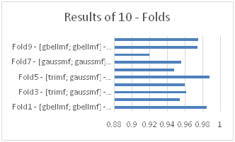
Figure 4 Results the best R²  of matrix MN in each fold.

ANFIS model on Taniguichi data

The purpose in this section is the same as above but we used with different data and features. We used four features: GC, CAI, rare codon frequency, AT for ANFIS model. For a membership functions set, we used again membership function in Table 2 and Gaussian combination membership function combined by two Gaussian membership functions.

Assumed that membership functions as MF and the number of fuzzy sets as NF, we have formula (10).

$MF=\{trimf,gbellmf,gaussmf,gauss2mf\}$

$NF=\text{{}i\in N\text{|}1<i<6\}$  (10)

The length test set of MF is 28. And the length test set of NF is 28. Thus, we have a matrix for training and testing MF and NF named as MN has a size 28×28. However, triangle membership function had an error when we selected for one of following features: GC, CAI, or rare codon frequency. Thus, the matrix MN was reduced to a size 9×28. In the overall matrix MN, the correlation coefficient between the model and the data is less than 0.6 (Figure 5).

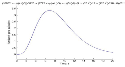
Figure 5 Using Chi – square pdf as the feedback function for modeling the gene activation stage.

FDEs model

Suppose $k=8,P_{on}=0.7,{\lambda }_1^{-}=0.4,{\lambda }_3=0.8,n_1^{\max }=44$ in equation (5) with $t\in [0,20]$ . We tested each probability distribution function P(t) for choosing the feedback function. We then figured out that the Chi – square distribution is the best fit to our conditions in equation (4) and equation (5), as shown in Figure 6, and formula (11).

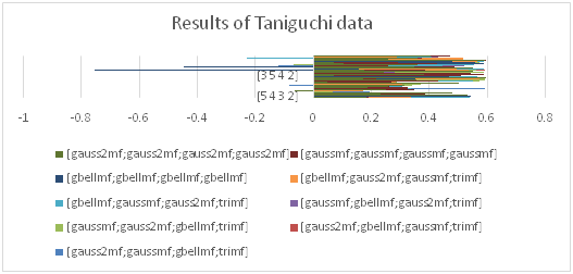
Figure 6 Results R² of matrix MN in Taniguichi data.

$f_{Chisquare}=f\left(t,k\right)=\frac{t^{\frac{k}{2}}{e}^{-\frac{t}{2}}}{2^{\frac{k}{2}}\text{Γ}\left(\frac{k}{2}\right)},t\ge 0$

Let $h=44,{\lambda }_1^{-}=0.4, P_{on}=0.7,$ and $n_2=100$  in equation (6) with $t\in \left[0,20\right]$ . Figure 7 is the graphs of our modified model.

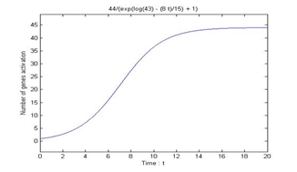
Figure 7 Using population growth as the feedback function for modeling the gene activation stage.

With the results above, to use equation (7) for solving the equation (7). Figure 8 is the result of the equation $n_1\left(t\right).$  To build fuzzy of inference system, we chose three fuzzy sets for each input and output named as: Low, Medium, and High. We used matrix – rules to create fuzzy rules for the system, as shown in Table 3.

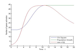
Figure 8 The graph of the equation $n_1\left(t\right).$

We chose triangle membership function which is the simplest membership function to use, as shown in formula (12) and Figure 9.

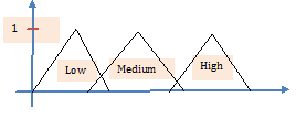
Figure 9 Triangle membership function.

$trimf\left(x;a,b,c\right)=\{\begin{array}{c}0, x\le a\\ \frac{x-a}{b-a},a\le x\le b\\ \frac{c-x}{c-b},b\le x\le c\\ 0,x\ge c\end{array},\forall x\in R$

$\begin{array}{l}\in R\\ a<b<c\\ a,b,c\in R\end{array}$ (12)

Finally, to get an exact value from FIS, we used mean of maximum (MOM) defuzzification method, the formula (13).

$n_2=\frac{{{\displaystyle \sum }}_{i=1}^{n_{fuzzy}}{\mu }_i*y_i^{max}}{{{\displaystyle \sum }}_{i=1}^{n_{fuzzy}}{\mu }_i }$  (13)

Where $n_{fuzzy}$  stands for the number of fuzzy sets, ${\mu }_i$  the calculated membership of the rule to the fuzzy set i and $y_i^{\max }$ is the expression value where the membership function of set i is at its maximum.

Our FDEs model depended on four parameters: the rate gene off ${\lambda }_1^{-}$ , the probability of gene on $P_{on}$ , the synthesis protein rate ${\lambda }_3$  and the rate of the average lifetime of proteins ${\tau }_3$ . In order to create, the FDEs model also has a parameter depends on the conditions in the gene. We modified and added a ANFIS system at translation stage with output is a rate of protein synthesis ${\lambda }_3$ . To test the new model, we choose random 70% of the data to train and the remaining of the data for testing and using cross-validation K-Fold with $K=10$ . Additionally, we change time $t\in \left[0,\alpha \right),\alpha \in N\backslash \left\{0\right\}$ in the model to test what is the good time t will give us a good result in Taniguchi supplement data. Generally, all of correlation coefficient values between the prediction values and original values are less than 0.2 in Table 4.

Gene optimization

We conducted optimized for protein-coding genes Prochymosin on Escherichia coli expression system BL21 with population size is 1000, mutate probability is 0.01, and cross – probability is 0.6. In genetic algorithm, we used ANFIS model built on Welch data as a fitness function for searching method. Results are shown in Table 5.

One of the main goals of this experiment was to attempt to find a way to create a model that can deal with missing information in data and a process that can solve differential equation when it missed information.

In results section of ANFIS model, we figured that our model adapted well to Welch data than Taniguchi data. In addition, we tried to use and add two new features in gene which are AT–rich and rare codon frequency. However, the results of the model are still low.

In FDEs model, we tested the system in Taniguchi data and the results did not have a good performance. The limited of this model is hard to find the data that can support enough information for analyzing and evaluating. Our model depends to six parameters. Based on biological theory, the parameters are gotten to some values. However, the synthesis rate λ_3 is found in experiment. This is the reason why we did not give more testing to modify the model. A greater understanding and evaluating of our findings could be a new approach in solving differential equation.

Based on the results in ANFIS model and FDEs model, we chose ANFIS model created by Welch data as the “fitness” function in genetic algorithm. A study by Menzella (HG, 2011) found some genes in Escherichia coli had a high gene expression. We chose the gene named as V2-pV2 in Menzella research to compare and optimize in gene optimization. In Table 4, the optimized gene in our research had a gene expression value larger than sequence V2-pV2. Moreover, the CAI value in our optimized gene showed us that the gene has a high CAI value which do not surely has a high gene expression and otherwise.

As mentioned in the Introduction, our purposed is to learn missing knowledge and information missing in data. The importance of our results is to use our model to approach and analysis information or pattern missing both in data and in solving differential equation.

We assessed the missing information both in data and in differential equation by using adaptive fuzzy inference system and fuzzy differential equations. Various combinations for features (CAI, GC, AT and rare codon frequency) in gene, rate of synthesis protein, and data were evaluated and analyzed using ANFIS model and FDEs model. The results in ANFIS model for Welch data showed us an ability to learn and predict value from missing information in data. We also believe that the system of FDEs model is a new estimate and compute differential equation in process of computation. We hope that our findings may influence machine learning and mathematical modeling. Future work will entail refining our model by looking for new data contains essential information for FDEs model and new feature in gene (e.g. mRNA secondary structure) for ANFIS model.

None.

The author declares no conflict of interest.

1. Palomares LA, Estrada MS, Ramire OT. Production of recombinant proteins: challenges and solutions. Methods Mol Biol. 2004;267:15–51.
2. Greene JJ. Recombinant Gene Expression. Totowa: Humana Press; 2004. p. 3–14.
3. Puigbo P, Guzman E, Romeu A, et al. OPTIMIZER: a web server for optimizing the codon usage of DNA sequences. Nucleic Acids Res. 2007;35(Web Server issue):W126–W131.
4. Dos Reis M, Wernish L, Savva R. Unexpected correlations between gene expression and codon usage bias from microarray data for the whole Escherichia coli K–12 genome. Nucleic Acids Res. 2003;31(23):6976–6985.
5. Bowden C. Analysis of enzyme kinetic data. Biochemical Education. 1995;23(4):225–225.
6. Heinrich R, Schuster S. The Regulation of Cellular Systems. Springer US; 1996. p. 1–372.
7. Voit EO. Computational Analysis of Biochemical Systems: A Practical Guide for Biochemists and Molecular Biologists. UK: Cambridge University Press; 2000. p. 1–544.
8. Zhang S, Wang RS, Zhang XS, et al. Fuzzy System Methods in Modeling Gene Expression and Analyzing Protein Networks. Fuzzy Systems in Bioinformatics and Computational Biology. 2009;242:165–189.
9. Dembele D, Kastner P. Fuzzy C–means method for clustering microarray data. Bioinformatic. 2003;19(8):973–980.
10. Vinterbo SA, Kim EY, Ohno ML. Small, fuzzy and interpretable gene expression based classifiers. Bioinformatic. 2005;21(19):1964–1970.
11. Zadeh LA. Is there a need for fuzzy logic? Information Sciences. 2008;178(13):2751–2779.
12. Effatia S, Pakdaman M. Artificial neural network approach for solving fuzzy differential equations. Information Sciences. 2010;180(8):1434–1457.
13. Tafti AD, Sadati N. Adaptive Neuro–Fuzzy Inference System in Fuzzy Measurement to Track Association. Dynamic Systems, Measurement, and Control. 2010;132(2):021009.
14. Sharp PM, Li WH. The codon Adaptation Index–a measure of directional synonymous codon usage bias, and its potential applications. Nucleic Acids Res. 1987;15(3):1281–1295.
15. McCall J. Genetic algorithms for modelling and optimization. Computational and Applied Mathematic. 2005;184(1):205–222.
16. Zadeh LA. Fuzzy Sets. Information and Control. 1965;8(2):338–353.
17. Negoita CV, Relescu DA. Applications of Fuzzy Sets to Systems Analysis. Springer Basel AG; 1975. p. 1–191.
18. Paulsson J. Models of stochastic gene expression. Physics of Life Reviews. 2005;2(2):157–175.
19. Bell G, Koufopanou V. The Architecture of the Life Cycle in Small Organisms. Philosophical Transactions of the Royal Society B. Biological Sciences. 1991;332:81–89.
20. Chen T, He HL, Church GM. Modeling gene expression with differential equations. Pac Symp Biocomput. 1999:29–40.
21. Welch M, Govindarajan S, Ness JE, et al. Design Parameters to Control Synthetic Gene Expression in Escherichia coli. PLoS One. 2009:4(9).
22. Taniguchi Y, Choi PJ, Li GW, et al. Quantifying E. coli Proteome and Transcriptome with Single–Molecule Sensitivity in Single Cells. Science. 2010;329(5991):533–538.
23. Menzella HG. Comparison of two codon optimization strategies to enhance recombinant protein production in Escherichia coli. Microb Cell Fact. 2011;10:15.