Conclusion: We define the Influenza Season 2013-2014 mathematically with the McNemar’s Test using the Laboratories’ real-time observations from the Americas, Europe/Asia, Africa and Australia/New Zealand. These real-time sequential frames from the weekly updated data show that
holds both for the normal and for the approximate standardized test statistics. We report live how this matched-pair model performs with the values of the interim missing data set to be zero, as these were the interim observations.
Introduction
The WHO Consensus on SARS in 2003 states, “centres were to relate clinical data on the onset in the symptoms and signs of SARS to viral shredding studies both retrospectively and prospectively” [1,2]. A textbook on mathematical statistics defines Complete Sufficient Statistics and the search for minimum variance estimators [3]. The “Current” Situation The opportunistic [4] airborne transmission of SARS could not get past the direct person-to-person small-particle aerosols transmission. The Avian Influenza
(H5N1) cannot as yet spread by small-particle aerosols [5] in human-to-human transmission. Standard surveillance for ILI’s [6], excess hospitalization [7], outpatient Visits [8], and traveling waves [9] do not explain the discrepancy between the simultaneous onset spread of geographically widespread outbreaks [10-12] and the inefficient transmission between person-to-person [10,13-15]. Worldwide stockpiling strategies are still being formulated [14,16] on how to improve the current strategy on vaccination and prophylactic anti-viral medications. The recent A (H1N1) situation in 2009_2010 reminds of the 1998 study [17].
Methods
The MATCHED-PAIR Relationship - the Null Hypothesis (Table 1) is that the moment to moment (i.e., real-time) changing or non-changing westerly (or northerly) winds have no relation with the distribution of the virus isolations within the geographic areas. This becomes a test for the matched-pair relationship [3]. The streamline flow or the turbulence [18] has no relation to the timing and the geographic location of the actual viral landings. From 2001 we used the log linear model ML estimate β to show the estimated probability that response on geographic location is x categories higher than the response on time equals exp (βx) times the reverse probability. From 2010_2011 we used the logit model β
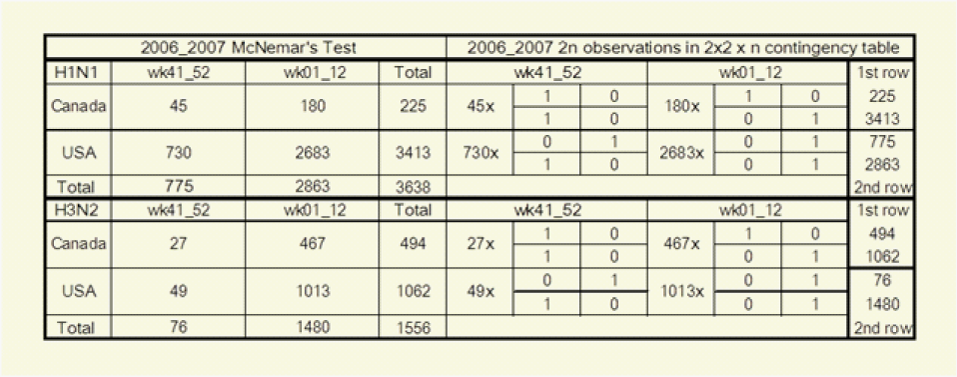
Table 1: McNemar’s Test and Cochran-Mantel-Haenszel Test collapsing the 2x2x n contingency table with n partial tables yields the marginal counts of McNemar’s Tests and each virus among n is match-paired with itself in its own partial table.
to denote a parameter for each subject the odds that the row response falls in category j or below (Instead of above category j) are exp (β) times the odds for the column response. The cross-classification in the above 2x2 Table (McNemar’s Test) where n=3638 actually presents 2n responses for the results of two surveys, those of the first survey in the horizontal row marginal counts and those of the second survey in the vertical column marginal counts. The Cochran-Mantel-Haenszel Tests on the above right present these same data differently as n=3638 separate 2x2 partial tables, one partial table for the two matched responses from each virus. Each 2x2 partial table has one column for each possible outcome, and the results of the first survey in row 1, and the results of the second survey in row 2 and collapsing the 2x2 x n contingency table for USA and Canada 11 yields the marginal counts of the McNemar’s tests.
The Missing Data
The 10-Region who/nrevss regional map contained the full version of the official data Regions. The 9-Region who/nrevss regional map showed how the observations could be missing or misplaced. The official 10-Region map carried the numbers (1-10) of the data Regions in bold and these numbers (together with their data) corresponded to the respective Regions in the 9-Region map, where Region 10 and its data were missing. We sequentially defined Regions 1, 10, (9-10), (8-10), (1-4) and (1-5) as further missing data and we presented these comparisons in the extreme conditions of. For weekly real-time computation we needed to define the entity of the interim missing data and which would be updated in the subsequent weeks.
Results
The McNemar’s Test and the Wald test (Proportional Odds Model)
On Figure 1-3 for Canada, Figure 4 for the US, Figure 5 for North America, Figure 6 for Europe/Asia, and Figure 7 for the Southern Hemisphere, we tested the matched-pair model generally with the standardized normal test statistic z of the McNemar’s Test on the upper left and compared this with the approximate z based on the Proportional Odds Model on the upper right. On the lower row within each graph we superimposed the 2x2 (2wk) and 4x4 (4wks) Tables to compare their real-time differences, A(H3) on the lower left and A(H1) on the lower right .
For Figure 2, the left upper diagram showed the full version of the official data (2x2 4wks) Row1/Row2=(7-10)/(1-6)=10R7 and (4x4 4wks) Row1/Row2/Row3/Row4 =Regions(910/78/56/1-4). The right upper (AH1), left lower (AH3) and right lower (B) diagrams showed the effects of the missing data (min and max) from both sides of Row1 or Row2 in the 2x2 Table Column(1, 2)=2w-wks. The three centre-most curves in each of these three diagrams were represented by 10R7=Row1/Row2=(7-10)/(1-6), 9R7 with out10=Row1/Row2 =(7-9)/(1-6) and 9R7 without1=Row1/Row2=(7-10)/(2-6). The upper boundaries were represented by 8R7=Row1/Row2= (7-8)/(1-6) and 7R7=Row1/Row2=(7)/(1-6. And the lower boundaries were by 6R7=(7-10)/(5-6) without Regions (1-4) and 5R7=(7-10)/(6) without Regions (1-5). With these missing data defined for Row1 the entire curves for 8R7=Row1/Row2=(7-8)/(1-6) and for 7R7=Row1/Row2=(7)/(1-6) moved upwards along the y-axis. The opposite occurred for Row1/Row2 =6R7=(7-10)/(5-6) without Regions (1-4) and for Row1/Row2=5R7=(7-10)/(6) without Regions (1-5). These moved downwards along the y-axis.
In Figure 3 we computed the full data from Canada, USA, as Row1/Row2=North/South = Canada/USA =BC-Atlantic/Regions (1-10) and the full data from Mexico, Guatemala and USA as Row1/Row2= South/North =Mexico-Guatemala/USA. For Canada/USA we computed these to be within the boundaries formed with Row1=BC- Atlantic Provinces without the Thunder bay data and with Row2=Regions (1-9) without Region 10. On the right upper graph the data were Row1/Row2/Row3/Row4 = Canada woont/ Ontario/ Region (125810)/Region (34679). In comparing the 2x2 Table with the 4x4 Table it was found that the original Row1/Row2 boundary should be kept intact as the Row2/Row3 boundary. For the Same reason the 2x2 Table for Mexcio-Guatemala/USA was compared with Row1/Row2/Row3/Row4 = Guatemala/ Mexico/ Regions (34679) / Regions (125810).
Figures 4 and 5 The McNemar’s Test and the Proportional Odds Model
The full version of the data represented by 10R7=Row1/Row2=(7-10)/(1-6) were computed to be within the two boundaries set between 9R7(without 10)= Row1/Row2 = (7-9)/(1-6) and 9R7 (without 1) = Row1/Row2 =(7-10)/(2-6). From a higher vantage point we computed the whole of North America with row1/row2 = Canada-Regions (125810)/Regions (34679)-Mexico-Guatemala and with row1/ row2/ row3/ row4 =Canada/Regions (125810)/Regions (34679)/Mexico-Guatemala in (Figure 5).

Figure 1: The McNemar’s Test and the Wald Test for Virus Isolation Data.
2014 wk 39 Canada. Left upper, Col (1,2)= 1wk, and right upper, Col(1,2,3,4)=1wk. Z on left is standardized normal statistic. Zpropodd on right is approximate z from proportional odds model. On left(for upper) are for full version Canada data computed within the boundaries set by the missing data from row1 and row2 of the 2x2 Table. Right(for upper) 4x4 Table showed the computations for all Canada data within the boundaries set without the Saskatchewan data in Row3.In the lower left, data for A(H3) (2x2) with and without sask data in Row1 compares with A (H3)(4x4) with and without sask data in Row2. On right lower, A(H1) both 2x2 and 4x4 superimposed.
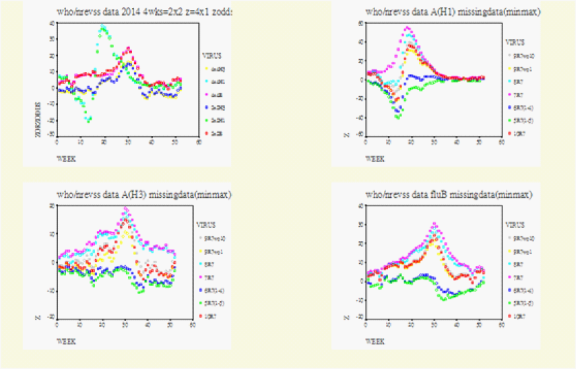
Figure 2: The Missing Data (minimized and maximized).
USA Season 2013_14 year to wk39.Left upper, z(2x2) for Col(1,2)=2wks and zodds(4x4) for Col(1,2,3,4)=1wk, and zorzodds is either z or zodds (approximate z). z is normal test statistic row1/row2=(7-10)/(1-6)=10R7 and approximate z (zodds) is for row1/row2/row3/row4=Regions(910/78/56/1234). For right Upper (H1), left lower (H3), and right lower(B), Col(1,2)=2wks, and 10R7=Regions(7-10)/(1-6), 9R7wo10 =(7-9)/(2-6), 8R7=(7)/(1-6), 6R7(1-4) =(7-10)/(5-6)= 6R7 without(1-4), 5R7=(7-10)/(6) without (1-5). For these three figures, missing data in row 1 elevate z, and in row 2 they lower z.
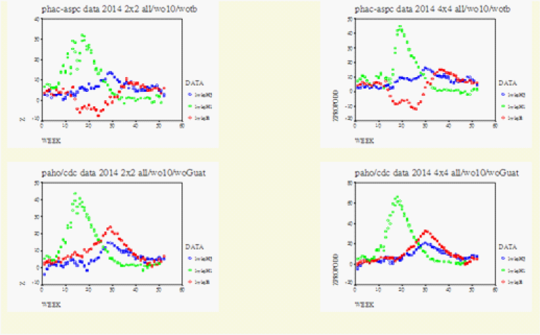
Figure 3: Row1/Row2=Canada/USA and Row1/Row2=Mexico-Guatemala/USA.
North American Season 2013-14 year to wk 39 Matched-pair behaviour. Upper. Row1/Row2=Canada/USA on left. Row1 from the left become on the right Row1/Row2=Canada woOt/Ontario.
Row2 From the left becomes on the right Row3/Row4= Regions(125810)/Regions(34679). Lower Left. Row1/Row2=Guatemala. Mexico/USA.
This Row1 become on the right lower Row1/Row2=Guatemala/Mexico. Row2 on the left lower becomes Row3/Row4=Regions (34679)/Regions(125810) on the right lower z is normal test statistic of McNemar’s Test. Zpropodd is approximate z of the proportional odds comparison of margins (4*4)
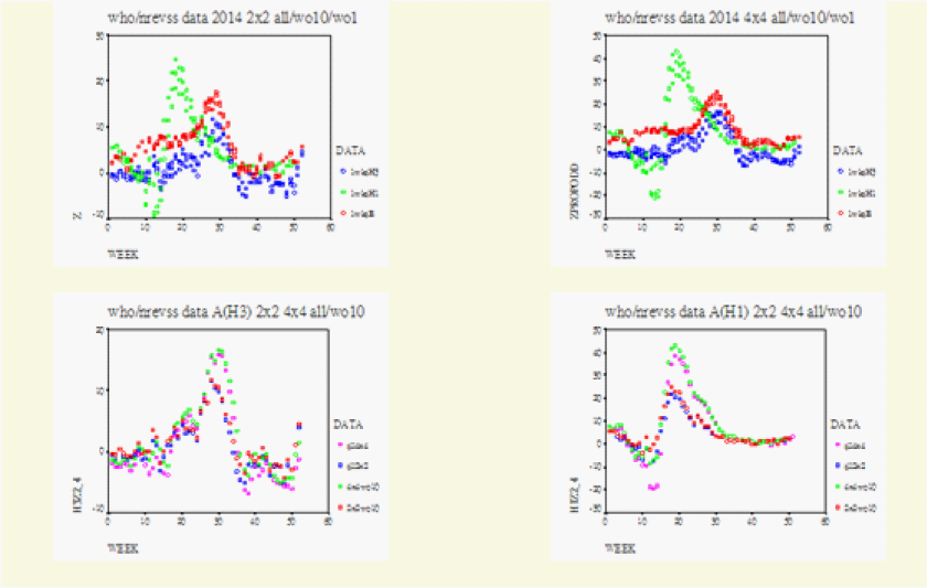
Figure 4:The McNemar’s Test and the Proportional Odds Model.
2014 US wk39. Upper Row compares the general matched-paired between the 2*2 and the 4*4 Tables. On left column (1,2)=1.week compares with right column (1,2,3,4)=1.week. z on left is standard normal static. Zpropodd on right is approximate z from proportional odds model. The upper left and the right are for full version 10 Regions computed within boundaries set by the missing data as defined. For the lower row each graph compares the specific matched-pair behaviour between 2*2 (2wks) and the 4*4 (4wks) Tables. Left is A(H3) and right is A(H1).

Figure 5:The McNemar’s Test and the Proportional Odds Model.
N America 2014 wk 39. Upper Row shows the general matched-pair behaviour between the 2*2 and the 4*4 Tables. Left Row1/Row2=Canada. Regions (125810)/Regions (34679). Mexico-Guatemala Row1 from the left becomes on the right Row1/Row2=Canada/Regions (125810). Row2 from the left is now on the right Row3/Row4=Regions (34679)/Mexico-Guatemala. Left upper, z is normal test statistic of the 2*2 Table. Right upper, zpropodd is approximate z of the 4*4 Table. Lower Row, on each graph the specific matched-pair behaviour between the 2*2(2wks) and 4*4(4wks): A (H3) on the left and A(H1) on the right.
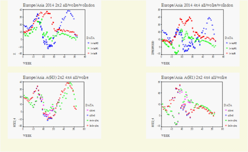
Figure 6:WHO data for Europe/Asia.
Europe/Asia 2014 wk39 Upper Row shows the general matched.pair behaviour between the 2*2 and 4*4 Tables. Left Row1/Row2=Europr/Asia. Row1 from the left becomes on the right Row1/Row2=Iceland_British_Isles/Contonental_Europe. Row2 from the left is now on the right Row3/Row4=Continental_Asia/Japan_Philippines_Indonesia. Left upper, z is normal test statistic of the 2*2 Table. Right upper, zpropdd is approximate z of the 4*4 Table. Lower Row, on each graph the specific matched.pair behaviour between the 2*2(2wks) and 4*4 (4wks): A (H3) on the lower right.
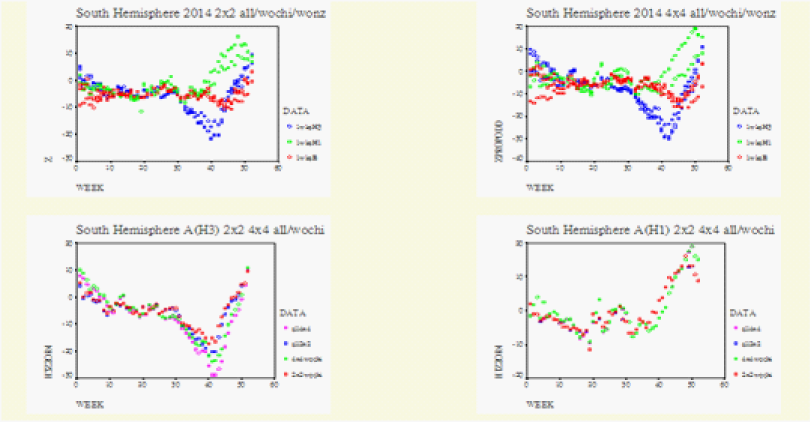
Figure 7:WHO data for the Southern Hemisphere.
Southern Hemisphere 2014 wk39. Upper Row shows the general matched-pair behaviour between the 2*2 and the 4*4 Tables. Left Row1/Row2=South_America_Africa/Australia-New Zealand. Row1 from the Left is on the right Row1/Row2=South America/Africa. Row2 from the left is now on the right Row2/Row4=Australia/New Zealand. Left upper, z is normal test statistic of the 2*2 Table. Right upper, zpropodd is approximate z of the 4*4 Table. Lower Row, on each graph the specific matched. Pair behaviour between the 2*2(2wks) and 4*4(4wks): A(H3) on the lower left and A(H1) on the lower right.
The Geographic Asymmetry by 4x4 Squared Tables
We examined the west-to-east symmetry coefficients from week 40 onwards from 2001_2002. The 4x4 Squared Tables was applied weekly to examine the symmetry of the floating 12_week average. For convenience we divided the Seasons into those dominated by A(H1N1) and those dominated by A(H3N2).
The Seasons dominated by Influenza A(H1N1)
The initial analysis with the 4x4 table between 2001 and 2008 showed that the symmetry coefficients for A (H1N1) were different from those for A(H3N2). There were three A(H1N1)-dominated Seasons and their maximum symmetry coefficients ranged from 0.8335 (2002_2003), to 1.0576 (2008_2009) and to 1.2744 (2006_2007). The average was 1.06, and this was much lower than 2.18 which was the average for the five A (H3N2) Seasons.
Season 2002-2003
For the major part of the Season A (H1N1) appeared to have positive symmetry coefficients. The symmetry coefficients for A (H3N2) appeared less positive and they seemed to be catching up with a steeper slope. At the end of the Season all the coefficients were converged together. This was the year when the hybrid A (H1N2) was reported.
Season 2006-2007
In the US we found that A(H3N2) behaved differently from A(H1N1). For Influenza A(H3N2), the symmetry for weeks 01 to 12 OR=0.62(0.57, 0.68) showed no change from OR=0.39(0.23, 0.67) for weeks 41_52. This difference can be examined more closely by the weekly computations. The scatter diagram of the weekly symmetry coefficients for A(H1N1) closely resembled that for A(H3N2) but Influenza A(H1N1) had a 6-8 week lead ahead of A(H3N2). This 6-8 week lead was reflected at the weekly ratios of H1 to H3 antigens. The cdc ratios for H1 to H3 antigens were decidedly elevated at 10/1 for week 49, at 99/7 for week 6 and 296/40 for week 12. On the background of this increased H1/H3 ratio only in the US, we found that it was not just simple coincidence that the west-to-east trajectory of Influenza A(H1N1) was increasing in the US from OR=0.76(0.65, 0.91) for week 41_52 to OR=1.95(1.82, 2.1) for weeks 01_12. We summarized the evidence for this difference with the McNemar’s Test for Canada/USA between Influenza A(H1N1) and Influenza A(H3N2). A(H1N1) had counts z=(180/730) /(180+730)^0.5=-18.23. The same test for A (H3N2) had counts z=(467-49)/ (467+49)^0.5=18.4. There was very strong evidence and probability for the A (H1N1) isolations to increase towards the US.
The Influenza A(H3N2) Seasons
A (H3N2) was dominant for 2001_2002, 2003_2004, 2004_2005, 2005_2006 and 2007_2008. Except for 2007_2008 the symmetry coefficients for A(H1N1) were difficult to compute. For Season 2007_2008, A (H1N1) showed a pattern identical to that for A(H3N2). These five Seasons had their maximum symmetries ranging from 1.62 to 2.98 with an average of 2.18. Except for Season 2005_2006, which had the lowest symmetry coefficient at 1.6230, all had increased excess mortality.
Season 2001_2002: The symmetry coefficients for A (H3N2) remained close to the maximum level around +2.0740 from weeks 05_16 to 08_19. The symmetry coefficients for Influenza A (H1N1) could only be briefly computed at 0.7082 at week 04_15. The coefficients for Influenza B remained negative throughout from week 40_51 to week 06_17.
Season 2003_2004: This was the year that was noted for the early and prolonged respiratory complications. The negative symmetry coefficients for A (H3N2) were converted positive very early at week 43_01 to +0.2267. These remained at 2 or above 2 from week 44_02 onwards to week 06_17 and peaked at 2.9851. During this period from week 43 to week 46 the drift variant A/Fujian/411/2002 arrived at the US and Canada.
Season 2004_2005: For this Season the symmetry coefficients converted from negative to +0.2368 between weeks 50_09. This peaked at week 05_16 at 1.6407. The A/California/7/04 arrived the US during week 2 and to Canada and Europe in week 07. By week 16 the mass migration was complete and A/California/7/04 had all but displaced the A/Fujian/411/2002.
Season 2005-2006: Among the five A (H3N2)-dominated seasons this Season had the lowest symmetry coefficient, 1.6230. This was the season without increased excess mortality.
Season 2007-2008: A(H3N2) showed a massive increase in their west-to-east asymmetry OR=14.1(12, 16.6) from OR=0.1(0.08, 0.14). Compared with 2003_2004 where the maximum coefficient was 2.985, the symmetry coefficients for Season 2007_2008 were converted to positive values late in the Season. Once converted onto positive territory however, these symmetry coefficients of the 2007_2008 Season increased very quickly to +2.5784 at week 09_20. Increased excess mortality was reported and this occurred late.
Season 2007-2008: A(H3N2) showed a massive increase in their west-to-east asymmetry OR=14.1(12, 16.6) from OR=0.1(0.08, 0.14). Compared with 2003_2004 where the maximum coefficient was 2.985, the symmetry coefficients for Season 2007_2008 were converted to positive values late in the Season. Once converted onto positive territory however, these symmetry coefficients of the 2007_2008 Season increased very quickly to +2.5784 at week 09_20. Increased excess mortality was reported and this occurred late.
Viral actions in Hong Kong by Matched-Pair Regression (Figure 8): We also performed matched-pair regression based on the surveys from authenticated but anonymous questionnaires from well-defined responders, which were found to be reliable and accurate [19-22].
Randomization and Sampling
Simple Random Sampling [22] to Hong Kong’s actively practicing N=3,000 doctor population, n=100 to n=200 questionnaires were sent every week to surveys on the symptoms and complications of Influenza-like-Illnesses, i.e., fever [yes/no], cough [yes/no], dyspnoea [yes/no], pneumonia [yes/no], diarrhea [yes/no] and patient’s history of contact with ILI’s [yes/no]. Institutional community clinics were included. Overseas addresses were excluded.
Mathematical Model for Regression Analysis
The model is an example of mixed model, containing the random effect i (intercept) and the fixed effect.(β)For PROC GLIMMIX, the outcome ‘1’ is ‘success’ and outcome ‘0’ is ‘failure’ for the response of pneumonia in the univariate 2-stacked data format. Let ψi denote the probability of a success for subject i’s response:
Equation 2 ai in the intercept representing an unobserved sample from a probability distribution, presumed to be normal distribution with unknown mean and standard deviation. Response (event=‘1’) denotes the probability of a success for subject is response; β1,β2,β3,β8 are coefficients for weekly respiratory virus isolations; Estimator = H1N1, H3N2, B, C, PFLU, MYCO, rsv, virus*virus. fh1, fh3 and fb are H1N1, H3N2 or b expressed as fraction of samples; contact number of patients per week who develop ILI’s after contact with other patients who had ILI’s.
We re-computed our data with PROC GLIMMIX from December 2004 onwards. We performed univariate regression analysis for pneumonia using Response (event=1), ‘1’ being success and ‘0’ being failure for pneumonia. The two response parameters of ‘pneumonia’ (binary) and ‘contact’ (Poisson) were stacked in the 2-tiered univariate format [23]. We computed the random (ai) effects and the fixed (β) effects for the different components of Virus Isolation Data 2004-2009 in accordance with our model, and Probability =
for “Response(event=1)”, this being the subject-specific effects from the i
th questionnaire and ith partial table of the McNemar’s Test. Note: Model is modified from PROC GLIMMIX documentation [23,24].
The McNemar’s Test and matched-pair data provided the model for this survey for matched-pair data, ‘1’= success and ‘0’=failure for ILI pneumonia. PROC GLIMMIX computed the random (ai) and fixed (β) effects for A(H3N2) and A(H1N1).
We define
as the subject-specific-effects from the ith questionnaire and partial table. We defined the five “core” Seasons from 2005 to 2009 to be: February_May 2005 Influenza A (H1N1) with the probability for success=‘1’ for pneumonia with the ith questionnaire pi=0.0203, =533; December_March 2006 with pi=0.2621 for
A(H3N2) and
=261, January_April 2007 with pi=0.9729 for A(H1N1) and
=2,202, February_April 2008 with pi=0.9327 for A(H3N2) and
=38 and the current Season February to April 2009 pi=0.1679 for A(H1N1) and
=2,962.
Multicollinearities
We defined that multicollinearities existed when the condition numbers were above
=2,962. As we plotted the log of the condition numbers between the subtypes A(H3N2) and A(H1N1) on the x-axis against their coefficients on the y-axis we found that the coefficients for the five “core” Seasons had formed a horizontal line indistinguishable from the x-axis. On the right beyond the log for the condition number
=2,962, we found the coefficients for the two subtypes A(H3N2) and A(H1N1) to be visibly diverged from each other. These diverged coefficients were from the two pre-Season periods, the first one being January to March 2005 for A(H3N2)
=51,121 and second one from January to March 2008 with the condition number
=807.53/0.000011. The diverging coefficients also came from the three post-Season periods April to June 2006 for A (H3N2)
=6,776.93/0.19 =35,668, February to May 2007 for A(H3N2)
=4,801.89/0.45247=10,613 and May to July 2008 for A(H1N1)
=3321/0.049 = 67,439.

Figure 8:The McNemar’s Test and the Proportional Odds Model.
N America 2014 wk 39. Upper Row shows the general matched-pair behaviour between the 2*2 and the 4*4 Tables. Left Row1/Row2=Canada. Regions (125810)/Regions (34679). Mexico-Guatemala Row1 from the left becomes on the right Row1/Row2=Canada/Regions (125810). Row2 from the left is now on the right Row3/Row4=Regions (34679)/Mexico-Guatemala. Left upper, z is normal test statistic of the 2*2 Table. Right upper, zpropodd is approximate z of the 4*4 Table. Lower Row, on each graph the specific matched-pair behaviour between the 2*2(2wks) and 4*4(4wks): A (H3) on the left and A(H1) on the right.
Co-circulations
We defined co-circulations to include our computed conjoint regressor A (H1N1)_A (H3N2) as per our mathematical model. In this format the two sub-types were truly “moving with each other”. The coefficients for these conjoint regressor A (H3N2)_A(H1N1) did not seem to be inflated by the multicollinearities (“moving with each other”) and they seemed to link up the different components of the Season.
The Baseline in 2005
For 2005 we did not compute any coefficient for our conjoint regressor. In addition the pi’s for pneumonia for both A(H3N2) and A(H1N1) during the pre-Season part (January_March 2005) and during the “core” part (February to May 2005) of the Season were zero or very close to zero OR=1.82(1.14, 2.90) pi =0.020. For the rest of 2005 the random (
) effects were very low, from -17.1951 to -6.1811. We therefore defined this period to be our baseline OR=0.73(0.61, 0.87) pi=0.0015 for A (H3N2) and OR=1.64(1.11, 2.42) pi=0.0034 for A (H1N1).
The entire Season (the expanded outbreak)
By “an expanded outbreak” we referred to the entire “Flu Season”. For 2005, 2006 and 2007 we found the expanded outbreak to include the core Season plus either one of the two other components of the “Season”, i.e., the pre-Season plus the core Season or the core Season plus the post-Season. For 2008 the entire “Flu Season” consisted all three components, the pre-Season, the core Season and the post-Season.
The tug-of-war/stalemate between 2006 and 2007PROC GLIMMIX provided a method for us to examine in detail the period between the 2007 and 2008 outbreaks. Using the weekly data for July_October 2006 the ith probability for success ‘1’ for pneumonia for A(H3N2) was pi=0.9338. Low 95% was pi=0.9315. These numbers for A(H1N1) was pi=0.9299 High 95% was pi=0.9302. Using the monthly data from this same period (July_Oct) the ith probability for success ‘1’ for pneumonia for A(H3N2) was pi=0.9843. Low 95% was pi=0.98335. These numbers for pneumonia for A (H1N1) was pi=0.9827. High 95% was pi=0.98327. The weekly data for Sept_Dec 2006 showed that this stalemate continued till the end of December 2006 when the ith probability for success ‘1’ for pneumonia for A(H3N2) ended at pi=0.9962. Low 95% was pi=0.9956. The same numbers for A (H1N1) was pi=0.9911. Its high 95% range was pi=0.9920.
Season 2006_2007 – the surge/resurge of A(H1N1)
During the “Flu Season” of January_April 2007 we saw the pi probability for success for pneumonia for A(H3N2) reduced from pi=0.9863 to pi=0.9590 and the pi for A(H1N1) increased from pi=0.8347 to pi=0.9729. For May_August 2007 the pi for A (H1N1) continued to be higher than that for A(H3N2), whether based on the weekly data (pi=0.0114) or based on the monthly data (pi=0.1945). For May_Dec 2007 the pi could be computed for A(H1N1) pi=0.2375 but not for A(H3N2).
Season 2007_2008 – the late return of A(H3N2)
The conjoint co-circulations for A(H3N2)_A(H1N1) appeared in December 2007 and this continued into the monthly data from January to March as OR=1.19(1.01, 1.4) and from April to July 2008 as OR=1.02 (1.001, 1.04) without any divergence for A(H3N2) and A(H1N1) in data 1, 2, 3, 6, 9 and 14. For January_Mar 2008, we computed the condition number
=(eigen value max/eigen value min) =807.53/0.000011. At these astronomical levels for the condition numbers, Proc Glim mix gave the random (ai) effects of 335.66. The fixed (β) effects for A (H3N2) were (-102.77) and for A(H1N1) +42.5. We could not interpret these except to say that A (H3N2) and A(H1N1) had “moved with each other”. The 2007_2008 “Flu Season” had three components, the January to March pre-Season with high condition numbers and marked divergence, the February & April 2008 “core” Season with low condition number
=(1,618.95/42.47)=38.12 without divergence. The third component of the Season from May to July 2008 had the condition number
= (3,772.26/0.04187)=90,095. The β coefficients for the conjoint regress or A (H3N2)_A(H1N1) seemed to link the three components to form the same Season.
Pandemic Season 2008_2009
This Season was in fact an anti-climax when compared with 2007_2008. The period Nov_Feb brought in the increased condition number of
=6,024. Only the coefficients for the conjoint co-circulation A (H3N2)_A(H1N1) could be calculated. The three periods that followed, i.e., Dec_Feb, Feb_April and for Feb_May had minimal coefficients respectively 0.04361 0.031 0.01234 for A (H1N1) and -0.1436 -0.1416 -0.1072 for A(H3N2). From these we could define Feb_April as the ‘core’ Season and that the condition number log
=log(2,962)=7.99 could now be defined as the new upper limit without divergence of the regression coefficients. The respective probabilities for success=‘1’ for pneumonia with the ith questionnaire could then be represented by these periods Dec_Feb, Feb_April and Feb_May. These were 0.1557 0.1679 0.1784 for A(H1N1) and 0.1324 0.1451 0.1597 for A(H3N2). These showed a positive trend as well as an improving statistics of fit (Figure 8).
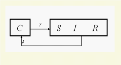
Figure 9:General Flow Diagram within the context of the matched-pair analysis, when the S, I and R compartments became indistinguishable from each other as β, the parameter for direct person-to-person contact transmissions, is in the limit of ⬬-0.
Discussion
In the face of the explosiveness of the 1918 influenza pandemic [24], the investigators were surprised to find that their estimates of the Basic Reproduction Number (R0) were much lower than expected. The investigators of the SIRC model defined the epidemiological parameters of (δ) and (γ) as the inverses of the average time spent by individuals in each of the compartments of R and C respectively [25]. Within the context of the 4x4 Squared Table, we think that the lower than expected R0 found for the 1918 pandemic should lead to the direction when (β) the parameter for direct person-to-person contact transmission was in the limit of :
Equation
Equation 3 shows that when the epidemiological parameter for direct person-to-person contact transmission (β) is in the limit of β-0 the compartments of S, I and R become indistinguishable from each other. The graphical form (Figure 9) resembles our everyday physical realities of the 4x4 and 2x2 Squared Tables.
The SIRC model defined (γ-1) and (δ-1) as the average time spent by individuals in each of the compartments of C and R respectively, and that the function represented the average age of a cross-immune individual, 25 and that they were inter-related [25,26]. Among the three levels (δ,and γ,and) of the time span factor in the original general flow diagram [25], we found one non-redundant dummy [19] variable beside (δ). We propose that one epidemiological parameter aside from the two epidemiological parameters (γ,δ) be needed for (Figure 9). At least one non-redundant epidemiological parameter should exist between the cross immune compartment and the single combined “SIR” compartment.
Acknowledgment
To the Department of Mathematics, Hong Kong Baptist University, Professor KT Fang, Professor Fred Hickernell and Professor SN Chiu.
References
- http://www.chp.gov.hk/guideline_sub78a9.html?id=267&lang=en&pid=119&ppid=97
- Consensus Document on the epidemiology of severe acute respiratory syndrome (SARS).
- Robert VH, Alen C (1995) Introduction to Mathematical Statistics. (5th edn), Prentice-Hal, USA.
- Roy Chad J, Milton DK (2004) Airborne Transmission of Communicable Infection-The Elusive Pathway. N Engl J Med 350(17): 1710-1712.
- Beigel JH, Farrar J, Han AM, Hayden FG, Hyer R, et al. (2005) Consultation on Human Influenza A/H5 (2005) Avian Influenza A (H5N1) Infection in Humans. N Engl J Med 353(13): 1374-1385.
- Fitzner K. A, McGhee SM, Hedley AJ, Shortridge KF (1999) Influenza Surveillance in Hong Kong: results of a trial Physician Sentinel Program. Hong Kong Med J 5(1): 87-94.
- Chiu SS1, Lau YL, Chan KH, Wong WH, Peiris JS (2002) Influenza-Related Hospitalizations among Children in Hong Kong. N Engl J Med 347(26): 2097-2103.
- Neuzil KM, Mellen BG, Wright PF, Mitchel EF, Griffin MR (2000) The Effect of Influenza on Hospitalizations, Outpatient Visits, and Courses of Antibiotics in Children. N Engl J Med 342(24): 225-231.
- Lin J, Andreasen V, Casagrandi R, Levin SA (2003) Traveling waves in a model of influenza A drift. J Theor Biol 222(4): 437-445.
- Dowell Scott F (2001) Seasonal Variation in Host Susceptibility and Cycles of Certain Infectious Diseases Emerging Infectious Diseases. Emerg Infect Dis 7(3): 369-374.
- http://www.phac-aspc.gc.ca/bid-bmi/dsd-dsm/rvdi-divr/index-eng.php http://www.chp.gov.hk/en/guideline_sub/97/119/267.html http://www.cdc.gov/flu/weekly/regions2009-2010/whousmap.htmhttp://www.cdc.gov/flu/weekly/regions2009-2010/hhswhousmap.htm http://www.who.int/influenza/gisrs_laboratory/flunet/en/
- Hammond G, Raddatz RL, Gelskey DE (1989) Impact of atmospheric dispersion and transport of viral aerosols on the epidemiology of influenza. Rev Infect Dis 11(3): 494-501.
- Stohr K (2005) Avian Influenza and Pandemics-Research Needs and Opportunities. N Engl J Med 352(4): 405-407.
- Alexander ME, Bowman C, Moghadas SM, Summers R, Gumel AB (2004) A Vaccination Model for Transmission Dynamics of Influenza. SIAM J Appl Dyn Syst 3(4): 503-524.
- Reichert T, Sugaya N, Fedson DS, Glezen WP, Simonsen L (2001) The Japanese Experience with Vaccinating School children against Influenza. N Engl J Med 344(12): 889-896.
- Balicer RD, Huerta M, Davidovitch N, Grotto I (2005) Cost-Benefit of Stockpiling Drugs for Influenza Pandemic. Emerg Infect Dis 11(8): 1280-1282.
- Bonabeau E, Toubiana L, Flahault A (1998) The Geographical Spread of Influenza. Proc Biol Sci 265(1413): 2421-2425.
- Haines K, Malanotte-Rizzoli P (1991) Isolated Anomalies in Western Jet Streams: A Unified Approach. Journal of the Atmospheric Sciences 48(4): 510-526.
- Agresti A (2007) An Introduction to Categorical Data Analysis. (2nd edn) John Wiley & Sons Inc., USA.
- Meier D E, Emmons CA, Wallenstein S, Quill T, Morrison RS (1998) A National Survey of Physician-Assisted Suicide and Euthanasia in the United States. N Engl J Med 338(17): 1193-1201.
- Asch DA, Jedrziewski MK, Christakis NA (1997) Response rates to mail surveys published in medical journals. J Clin Epidemiol. 50(10): 1129-1136.
- Scheaffer M, Ott L (2011) Elementary survey sampling. (5th edn), Duxbury Press.
- http://support.sas.com/rnd/app/da/glimmix.html
- Mills CE, Lipsitch M, Modeling the Transmission of Pandemic Influenza to Estimate the Basic Reproductive Number
- Casagrandi R, Andreasen V, Bolzoni L, Levin SA (2006) The SIRC model and influenza A. Math Biosci 200(2): 152-169.
- Pease C (1987) An evolutionary epidemiologic mechanism, with applications to type A influenza. Theor Popul Biol 31(3): 422-452.

© . This is an open access article distributed under the terms of the,
which
permits unrestricted use, distribution, and build upon your work non-commercially.


 World Malaria Day, observed annually on April 25SUP>th. The purpose of this day is to raise awareness about the global struggle to combat malaria, highlighting the need for continued research, prevention, and treatment strategies to eradicate this deadly disease. So, it is an opportunity to all the researchers to submit your interesting papers on raising the approachability on modern vaccine development, advances in disease control, prevention and eradication and the submissions received till April 25th, 2024 will be offered a best discount of 30% for publication in Journal of Human Virology & Retro virology.