The Monte Carlo calculation of integral dose shows its sensitivity in the treatment plan dose distribution and dose-volume histogram (DVH) variation. To take advantage of the efficiency of the integral dose objective function in treatment planning optimization, the sensitivity of the target shape to the integral dose in the treatment plan beam setup, and the arbitrary characteristics of the contouring method, we developed a statistical integral dose calculation method using a Monte Carlo integral dose computation algorithm. When the analytical dose distribution function is available, this Monte Carlo approach overcomes voxel size constraints and edge voxel approximations. Variations in the contours (e.g., expansion of the target) were analyzed, and their effects on the treatment plan beam orientation selection were shown. In this study, we first demonstrate the insufficiency of volume calculation for pixel or grid size based integral dose or volume especially for high resolution and certain size of target treatment. Then the Monte Carlo integral method was employed to calculate the integral dose. The effectiveness of this Monte Carlo calculation method was demonstrated by using a cubic target, a C-shaped target with a nearby cylindrical critical structure, and a clinical case involving eye-lens shielding. The results showed that it is important to consider the voxel size effect when evaluating treatment plan dosimetry and that the Monte Carlo Integral Computation algorithm can be an alternative to voxel-based integral dose calculation methods in accounting for up to 2 mm displacements of the critical structures, which can result in as much as a 28% variation in the treatment pattern. We suggest that integral dose be used as an objective function in treatment planning to adjust initial adaptive target radiotherapy and to generate initial blocking beam treatment patterns for Gamma Knife treatment. This approach will provide better treatment with fewer complications, especially in single fraction stereotactic radiosurgery.

Keywords: monte carlo, integral dose, gamma knife, stereotactic radiosurgery

IGRT, Image-guided radiation therapy; DVH, dose-volume histogram; GTV, gross tumor volume; CTV, clinical target volume; PTV, planning target volume; TPS, treatment planning systems; ROI, region of interest; LGP, leksell gammaplan

With new imaging technology and the increasing use of IGRT, the future development of treatment planning system will be based on artificially intelligent decision making. So called adaptive radiotherapy attempts to adjust the treatment plan by tracking small variations in the target volume (i.e., the GTV, CTV, or PTV). Sensitive object functions or optimization approaches are needed to reach this goal. Target shape variation is an important factor in that the migration of the tumor can adversely affect target dose delivery. Clinically, volume expansion from GTV to PTV is common in treatment planning systems (TPS). For example, the Pinnacle ADAC TPS¹ uses different contraction and expansion algorithms. If high level dose conformity is required, knowing the variation in volume due to the expansion is crucial. The method used to calculate the volume of the region of interest (ROI) is:

$V_{roi}=v\times \left(N_i+0.5N_e\right)$   (1)

where v is the size of voxels, $N_i$ is the number of inner voxels, $N_e$ and is number of edge voxels. Voxels of different sizes have different effects on the accuracy of the volume calculation. An intuitive approach to avoiding the grid size effect is to decrease the voxel size; however, when the voxel is smaller than a micro-meter, continuously decreasing the voxel size may negate the physical meaning of the micro-radiobiologic effect. Naturally, a method of volume calculation independent of the grid is needed. The Monte Carlo algorithm is an alternative method for accurate volume calculation and quality assurance, which can be used to avoid the effect of voxel approximation. Calculation accuracy can be controlled by the number of sampling points. In gamma knife blocking beam treatment planning, it has been shown that integral dose can be used as one of the sensitive object functions by combining information from three dimensions.^2,3

Calculation of integral dose is also affected by voxel size. Even though different methods are available to avoid inaccuracies due to pixel size deficiency, the physical constraints and approximations of the pixel approach limit its ability to express the real physical condition when the voxel size is smaller than the cells themselves. Therefore, in this study, we developed a Monte Carlo algorithm to calculate the volume and integral dose and compared its results with those of the pixel counting method. We also used the Monte Carlo integral dose object function to analyze variations in the target volume using a Gamma Knife treatment planning model.

In stereotactic radiosurgery, accuracy of dose delivery is crucial, especially for small targets. There are two issues associated with stereotactic radiosurgery. The first is treatment setup accuracy, and the second is calculation accuracy. Integral dose is an effective objective function in optimization of Gamma knife blocking beam treatments. The optimization of a Gamma Knife treatment plan is a complex problem that has elicited several different solutions.^4,5,6 However, most resultant optimization algorithms have been based on the pixel dose constraint because the Gamma knife treatment plan is determined by the shot center $\left(x,y,z\right)$ the weight of the shot, and the size of the collimators. This generates a multiple-variable optimization problem that can be solved using nonlinear equations and simulated annealing algorithms. In addition, the challenge of balancing the effects of the different variables makes the problem even more complicated. Introducing integral dose, which combines the target volume, shape, dose, and geometry information into one objective function, simplifies the process so that a fast search algorithm can be applied in finding an optimal plan. The integral dose also reflects the intrinsic correlation between the dose distribution and the target volume. Using integral dose in this way can improve the treatment plan by reducing computation time and increasing dosimetric precision.

The integral dose calculation accuracy is affected by the grid size definition; and, in the Leksell GammaPlan (LGP), the dose point is calculated as 31×31×31 voxels. The integral dose changes with changes in voxel size. Therefore, integral dose can be used to optimize blocking pattern treatments.^2,3 Calculation of integral dose involves two factors: target shape and dose distribution. Because different target shapes give different volumes, we first compared the volumes calculated using both the pixel counting method and the Monte Carlo method. Then, we used the Monte Carlo method to do the calculation using contours from a clinical case. The different results in blocking pattern treatments for the gamma knife system were analyzed. The calculated results were evident in pattern changes and in the DVHs.

In the Monte Carlo computation method, the number of sampling points affects the accuracy of the calculation. If the volume is calculated by counting the number of voxels inside the boundary, then the number of voxels determines the volume accuracy (i.e., the higher the number of voxels counted, the greater the accuracy). Therefore, we tried different voxel sizes in calculating the dose. Physically, the integral dose is the total energy absorbed by a specific volume of tissue. The clinical effect of this process is not clearly understood;⁷ however integral dose includes the whole radiation volume and may have some correlation with the radiation response of tissue abutting the high dose region. Therefore, the integral dose is an important factor in radiotherapy.

In calculating the integral dose and selecting of blocking beams in Gamma Knife treatment planning, we generally calculate each plug’s contribution to the dose per voxel or in the contoured region. The dose at a particular point D_i(x, y, z) receives contributions from different plugs, and the integral dose for a particular region can be calculated in two ways. One way is to calculate the integral dose that each plug contributes to the critical region C_R, and the other is to calculate the total integral dose I_i of all the plugs. This procedure is described by following Equation (2), which shows that the order of the integration procedure can be adjusted:

$I={\displaystyle \sum _{n-1}^{N}Ii={\displaystyle \sum _{n-1}^N{\displaystyle \underset{C_R}{\iiint }Di}}}\left(x,y,z\right)dxdydz={\displaystyle \underset{C_R}{\iiint }{\displaystyle \sum _{i-1}^{N}Di}}\left(x,y,z\right)dxdydz={\displaystyle \underset{C_R}{\iiint }D\left(x,y,z\right)dxdydz}$   (2)

Given that the integral dose of the target is controlled by the volume $V\left(x,y,z\right)$ of the region $CR$ and the dose distribution $D\left(x,y,z\right)$ , then integral dose I can be expressed as:

$I=I\left(V\left(x,y,z\right),D\left(x,y,z\right)\right)$

Then any variation of the integral dose I can be expressed as:

$\Delta V=\frac{\partial I}{\partial V}\Delta V+\frac{\partial I}{\partial D}\Delta D$

If $\Delta V=0$ is the condition necessary to preserve the clinical effect, theoretically or experimentally, it is worth analyzing the variations of V in adaptive radiotherapy. It is obvious that changes in result in changes in V the dose. The dose distribution is adjusted by turning the beam on and off, changing the length of time the beam is on, and adjusting the orientation of beam. It is interesting to calculate the volume variation that results from different factors such as target shrinking, target motion (or displacement), target deformation, density change, and so on. In other words, it is possible to induce the equivalent volume concept, which is like the concept of equivalent dose. The dose-volume effect depends on the accurate calculation of the volume. In this study, we applied the Monte Carlo method to devise an algorithm to calculate the volume variation effect on dose distribution and treatment planning in a gamma knife analytical dose model.²

There are several integral dose calculation methods that can be used to accomplish this objective. Because the integrated volume is determined by the contour, and knowing a point inside the contour is needed for both pixel counting method and Monte Carlo method to compute the integral volume, we first introduce the algorithm to check a point inside the contour, and then specify the methods for integration computation.

Algorithm to check arbitrary point inside a contour

The contour can be expressed as $\left\{x_{ij},y_{ij},z_i\right\}$ where $i=1$ to m, m is the total number of 2-dimensional layers, $j=1$ to n, and nis the number of contour points. Any point $\left(x,y,z\right)$ can be determined by checking whether it lies within a certain contour layer. To check if a point is within a contour, we employed the following method:

Given contour polygon point group $\left\{x_n,y_n\right\}$ in same slice, where $n\in \left[3,N\right]$ and N is an integer, which is larger than 3 (Figure 1). The algorithm to check point $P_{ijk}\left(x_i,y_j,z_k\right)$ in the polygon

can be expressed as pseudo code:

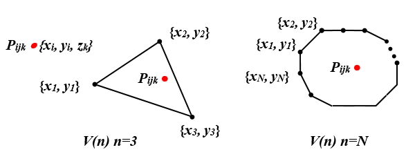
Figure 1 The method to check point P_ijk (x_i,y_i,z_i) inside the volume determined by polygon contour.

For a contour point set or graph expressed as $V\left(N\right)$ , and point $P_{ijk}\left(x_i,y_j,z_k\right)$ .

 Confirm that the points are inside the contour:

1. $T=0$  (point $P_{ijk}\left(x_i,y_j,z_k\right)$ is outside of $V\left(N\right)$
2. For any pair of points v₁ and v₂ in $V\left(N\right)$ , if the y coordinate of point $P_{ijk}\left(x_i,y_j,z_k\right)$ is within the range of the y coordinate of the contour range and at the right of the line formed by points v₁ and v₂, then $T=1$ ;
3. Return T;

Methods to compute the integration

1. The direct integration method

This method is simple and involves three steps:

1. Finding the range of x and y in the curves using an approximate analytical formula;
2. Integrating the analytical contour and multiplying by the slice distance t to get the slice volume V;
3. Totaling all the 2-dimensional slice volumes V to get the total volume integration.

However, the difficulty in finding the exact analytical representation of the target is a challenge. If the distance between the slices is too large, volume information may be lost.

2. The pixel counting method

1. Determine all point $P_{ijk}\left(x_i,y_j,z_k\right)$ from the minimum x and y directions in ranges $\left[X_{\min },X_{\max }\right]$ and $\left[Y_{\min },Y_{\max }\right]$ using the contour boundary point set $\left\{x_{ij},y_{ij},z_i\right\}$ ;
2. Verify that point $P_{ijk}\left(x_i,y_j,z_k\right)$ is inside the contour using the method described above;
3. Multiply the number of points $P_{ijk}\left(x_i,y_j,z_k\right)$ inside the contour by the number of voxels of grid size a. Then, the integral dose $I_D$ is:

$I_D=f{\displaystyle \sum _{i=o}^{N}d\left(x_i,y_i,z_k\right)}$

where N is the number of voxels inside the target volume, f is the scale factor, and the accuracy of the point dose $$d\left(x_i,y_i,z_k\right)$$ is determined by the grid size a.

3. The Monte Carlo method

1. Randomly generate point $P_{ijk}\left(x_i,y_j,z_k\right)$ within the range $\left[X_{\min },X_{\max }\right]$ and $\left[Y_{\min },Y_{\max }\right]$ as determined by the contour polygon boundary;
2. Verify that every point $P_{ijk}\left(x_i,y_j,z_k\right)$ is inside the contour;
3. Calculate the integration based on the relationship between the number of points generated and the number of points inside the contour.

More specifically, the algorithm can be represented by the following pseudo code:

1. Find the contour point range $\left[X_{\min },X_{\max }\right],\left[Y_{\min },Y_{\max }\right]$ ;
2. Define the whole region volume $V=\left(X_{\min },X_{\max }\right)*\left(Y_{\min },Y_{\max }\right)*t$ , where t is the thickness of the image slice.
3. Generate arbitrary points (x_i,y_i) randomly using the formula $x_i=X_{\min }+\left(X_{\max }-X_{\min }\right)*f_{ran},$ $y_{{}_i}=Y_{\min }+\left(Y_{\max }-Y_{\min }\right)*f_{ran}$ ; where $f_{ran}$ is a random fraction.
4. Verify that point $P_{ijk}\left(x_i,y_j,z_k\right)$ is inside the contour by the method described above;
5. Set the Integral dose as $I_D+=V*D\left(x_i,y_j,z_k\right)/n$ for all sampling points n

In this study, we analyzed several contours to illustrate Monte Carlo Integral dose calculation and described a clinical case. Initially, we tested Monte Carlo calculation based on a cube shaped volume. Then we tested integral dose sensitivity using a semi-circular cylinder. Finally, a case involving eye lens dose blocking beam treatment was included to show the effectiveness of the plugging pattern treatment plan generated by this Monte Carlo Integral dose computation method.

To guarantee the accuracy of our analysis, a series of procedures were followed to check the calculation. Our methodology was derived from analysis of a simple shape, a complicated structure, and a clinical case. And this approach guided us throughout the process of developing this algorithm. A cube was chosen to make certain that all voxels remained within the boundary of the polygon. We used the semi-circular cylinder because the circumference of a circle approximately represents an infinite number of sections of line. Then a clinical case was used to show the application of the Monte Carlo integral dose and the calculation benefit in the analytical Gamma Knife dose model. The Gamma Knife dose model can be calculated based on the measurement of the helmet and some of the reference points.⁸ The Gamma Knife C model dose simulation was verified by the profile comparison, which is shown in figure 2, where the 2-dimensional dose profiles can be seen along the x, ,y and z axes. The solid data point was directly extracted from the Leksell Gamma Knife Treatment Planning System (LGKTPS).

Figure 2 Simulation of Leksell Gamma Knife C model in x, y, z directions. The diamond points are the data from LGK TPS. The solid line is from the computed model.

Monte Carlo calculation for a cubic shape

Figure 3 shows the cube that we generated by simulating the frame coordinate system of the LGKTPS. The center of the cube coincides with the center of the frame (which is x=100, y=100, z=100); and the axial plane bisects the cube at Z=100. The cubic volume was fixed for testing purposes. The insufficiency of the pixel counting computation method was illustrated by calculating the volume based on grid size variations. Figure 4 shows the effect of grid size on the computation. Obviously, different grid (voxel) sizes generate different volume percentages for the cube, even though the grid size is large enough to cover the entire cube. In figure 4, the grid size was too small to cover the cube; therefore, it was possible that the calculated volume would be different from the full volume of the cube. In Figure 5, for the upper figure, the voxel size is set to 0.06 of the length of the edge of the cube. The calculation results in 289 voxels inside the boundary; and the voxel calculation method results in a volume that is about 104% of the cube. The lower figure shows that if the voxel size is set at 0.01 of the length of the edge of the cube, the resulting 961 voxels would cover only 38% of the real volume.

Figure 3 Cubic structure used for the volume calculations, based on 31×31×31 voxels with different grid sizes.

Figure 4 The circles show that the computed volume (i.e., the percentage of the volume of the cube) varies in relation to the voxel size.

Both scenarios can be avoided by using different approaches. For example, formula (1) offers a solution to the problem of the grid or voxel lying across or outside of the boundary of the volume, which is the situation shown in the upper of figure 5. The problem of insufficient coverage seen in the lower part of figure 5 can be avoided by a visual check. The Monte Carlo method is another solution for both scenarios, correcting them both by using a defined boundary larger than that of the given volume. This computation is more cumbersome when integration of a function is needed inside the defined boundary or target. More simply, when the number of sample points is increased, the Monte Carlo method can give an acceptable result, usually around ±5% or better. This phenomenon is also addressed elsewhere.⁹

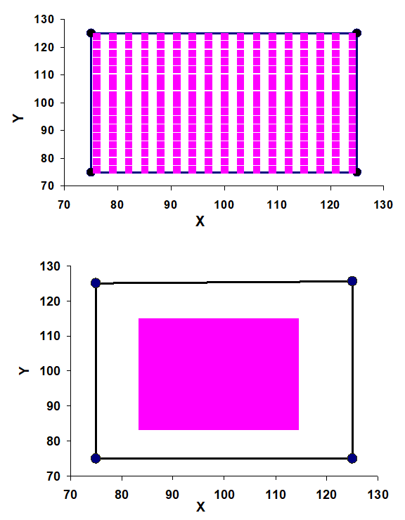
Figure 5 Illustration simulating the voxel size effect on the accuracy of volume calculations.

2. Monte Carlo calculation of the integral dose for a cylindrical half-ring target surrounding cylindrical critical structure

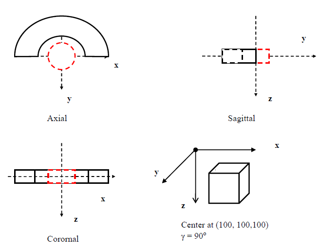
Figure 6 illustrates dose calculation using a half-ring target surrounding a critical structure as a cylinder at the center. This target was chosen because the circumference of a circle approximately represents an infinite number of sections of a line, which gives a general scenario. We defined the half-ring target as:

$\begin{array}{l}{r}_1<{\left({\left(x-o_x\right)}^2+{\left(y-o{}_y\right)}^2\right)}^{1/2}<r_2\\ Z_{down}<\left(z-o_z\right)<Z_{up}\end{array}$

Figure 6 A cylindrical half-ring as target with a cylinder critical structure.

where $r_1$ and $r_2$ are the inside and outside radii; $\left(o_x,o_y,o_z\right)$ is the center of the ring, and $Z_{down}$ and $Z_{up}$ are used to define the range of the axial direction. The cylindrical critical structure is defined as:

$\begin{array}{l}{\left({\left(x-o_x\right)}^2+{\left(y-o{}_y\right)}^2\right)}^{1/2}<r_c\\ Z_{down}<\left(z-o_z\right)<Z_{up}\end{array}$

where $r_c$ is the radius of the cylinder. To apply and evaluate our Monte Carlo Integral dose computation in Gamma Knife Plugging pattern treatment, we followed two steps: first, we checked the convergence of the Monte Carlo calculation, and then we tested its sensitivity as a treatment planning object function.

Figure 7 shows the sample point effect on the integral dose calculation by three different trials. The calculation converges at about 100,000 sample points. The number of sample points is determined using an exponential formula. In this setup, we used the integral dose that was calculated by the Monte Carlo method to test the target variation effect on the treatment plan. The Gamma Knife treatment planning system was selected due to the fixed number of beams (201) and fixed geometry of those beams. After checking the convergence of the Monte Carlo calculation, we employed this method to show the sensitivity of the integral dose in beam selection. We fabricated a nine shot Gamma Knife treatment plan with the shot centers midway between inside and outside rings. With a sequence blocking beam treatment for each shot selected, 24 beams were selected to block. There are different possibilities for target variation. A typical case would be the displacement of a target such as an organ at risk. Figure 8 shows three different blocking patterns. Figure 8(a) shows an original setup with 9 plugging shots. Figures 8(b) and 8 (c) show the plugging patterns after the critical structure has been shifted 2 mm superiorly or inferiorly. We developed several mechanisms to compare the different plugging patterns in both the DVH's and treatment patterns. In figure 9, the upper DVH shows the difference due to structure displacement. The circles represent the DVH of the critical region without displacement. The triangles represent the DVH resulting when the critical region is shifted superiorly 2 mm, and the squares represent the situation when the critical region is shifted inferiorly 2 mm. When a blocking beam pattern is used for the treatment, the DVH curves show two features: in one, the dose in the critical structure is significantly lower; in the other, the difference in the three DVH curves decreases and DVH curves nearly overlap each other due to selection of blocking beams. Obviously, displacement of the target leads to variation in the treatment setup. The target DVH curves are not shown because they are overlapped and almost identical for the given resolution in figure 9.

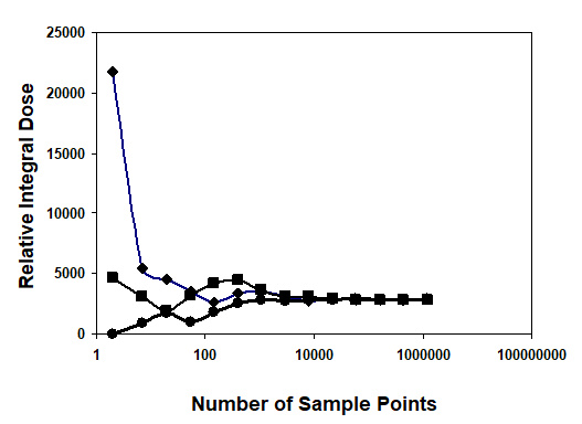
Figure 7 Illustration of the convergence of Monte Carlo Calculation of Integral Dose.

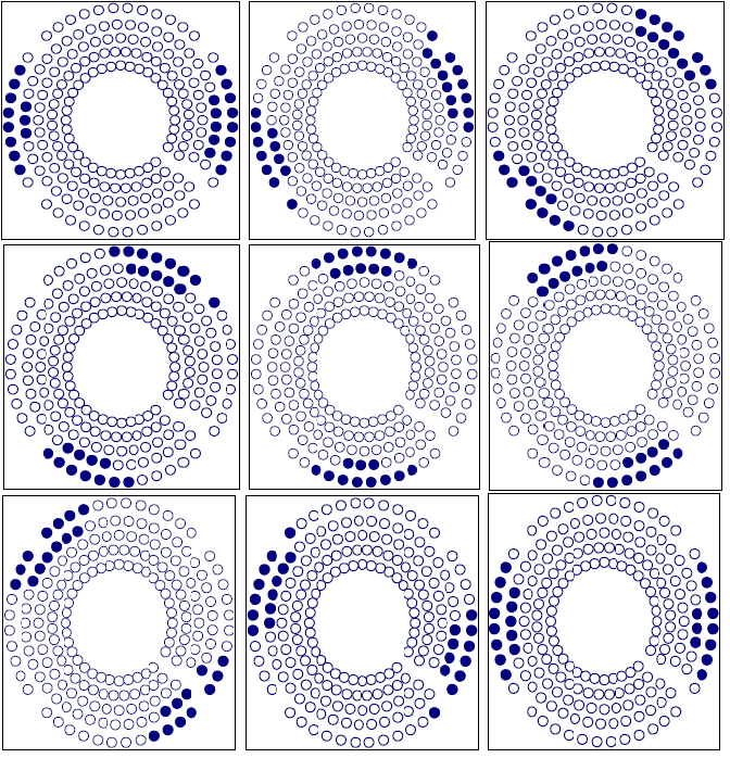
Figure 8a Plugging Pattern of a 9 shot treatment without displacement of the critical structure.

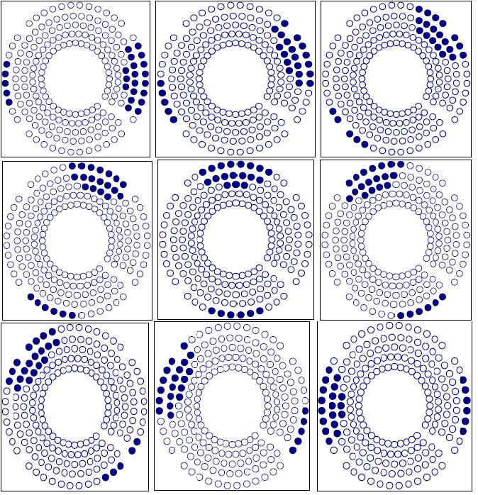
Figure 8b Plugging Pattern of a 9 shot treatment with the critical structure displaced 2 mm superiorly.

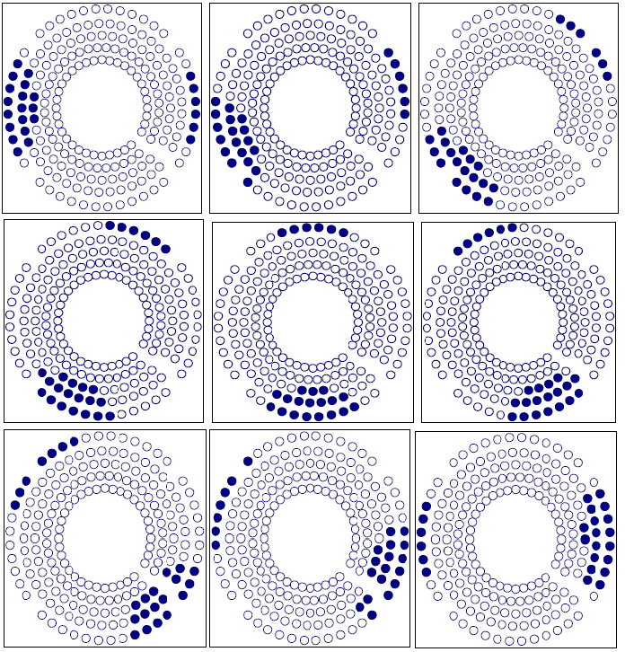
Figure 8c Plugging Pattern of 9 shots treatment with the critical structure displaced 2 mm inferiorly.

Figure 9 DVH curves from the cylindrical Critical Structures.

To show the significance of these differences in the treatment pattern, we devised a formula to describe the distortion. Given the two feature vectors $R_i$ , and $R_j$ for the two sets of treatment configurations, which is the plugging beam index, the distortion $M\left(R_i,R_j\right)$ can be expressed as:

$M\left(R_i,R_j\right)=\left|\frac{R_i-R_j}{R_i}\right|$

This calculation shows that the distortion is 28% when the critical region is shifted superiorly 2 mm, and distortion is 24% when the critical region displaced inferiorly 2 mm. The difference in these percentages is a result of differences in the helmet's distance from the target.

Monte Carlo calculation of the integral dose in a clinical case involving eye lens shielding during Gamma Knife treatment

Eye lens dose is a concern in radiation treatment of ocular cancer.^10,11 However, determining which beam should be plugged is difficult, especially when the eye lens is far away from the treatment target. Figure 10 illustrates such a circumstance. Combining the Monte Carlo integral dose model and the analytical dose model, we can easily generate a blocking pattern that will decrease the eye-lens dose by more than 50%. This result is shown in Table 1. In this case, we prescribed the dose to average center of the 9 shots. The critical structure was defined as the lens of the right eye, and reference point dose was prescribed to the center of this structure. The dose was decreased is up to 81.7% by selecting 3 beams to block. These data suggest that blocking beam selection is a mechanism that is sufficiently sensitive and effective for integral dose calculation. Therefore, the Monte Carlo integral dose calculation method can be an effective tool in selecting beams to block to protect organs at risk in Gamma Knife treatment plans.

Figure 10 Eye lens dose avoidance using Monte Carlo Integral dose calculation.

In this study, we investigated the relative effectiveness of the pixel-counting volume calculation method and a Monte Carlo algorithm in calculating integral dose in treatment planning. We found that, without careful selection of the location of the voxels and size of the voxels, the voxel-based method for calculating integral dose or volume may result in large variations. The Monte Carlo method is an alternative method that can be effective in avoiding these large variations. This Monte Carlo method can easily be implemented in treatment planning systems and provides a convenient tool for quality assurance.

Some shortcomings of the Monte Carlo method need to be addressed. For instance, variations in integral dose are generated due to the fluctuation of the random number generator. These variations could result in a 5% difference; however, this difficulty can be reduced by increasing the number of sampling points.

In our clinical example, we showed how variations in the target could affect a Gamma Knife blocking beam treatment plan. A 2 mm target displacement could generate a >28% variation in the treatment pattern, which emphasizes the importance of accurately defining the target for Gamma Knife stereotactic radiosurgery. This method of analysis could possibly be applied in external beam treatment planning as well, and quantitative measurement and analysis of integral dose will be next research step.

The authors express their gratitude to Robert Luo in pattern display program.

None of the authors have expressed any conflict of interest related to this study.

1. Pinnacle treatment planning manual, release 7.6.
2. Li K, Ma L, Selective source blocking for Gamma Knife radio surgery of trigeminal neuralgia based on analytical dose modeling, Phys Med Biol. 2004;49:3455–3463.
3. Li K, Ma L, A constrained tracking algorithm to optimize plug patterns in multiple iso–center gamma knife radiosurgery planning. Med Phys. 2005;32(10):3132–3135.
4. Yan Y, Shu H, Bao X, et al. Clinical treatment planning optimization by Powell’s method for Gamma Unit treatment system. Int J Radiat Oncol Biol Phys. 1997;39(1):247–254.
5. Wu QJ, Bourland JD. Morphology–guided radiosurgery treatment planning and optimization for multiple isocenters. Med. Phys. 1999;26(10):2151–2160.
6. Leichtman GS, Aita AL, Goldman HW. Automated Gamma Knife dose planning using polygon clipping and adaptive simulated annealing. Med Phys. 2000;27(1):154–162.
7. Mayneord WV. The measurement of radiation for medical purposes. Proc Phys Soc. 1942;54:405–421.
8. Marcu SM, Wu QJ, Pillai K, et al. GammaPlanÒ–Leksell Gamma KnifeÒ raidosurgery treatment planning verification method. Med Phys. 2000;27(9):2146–2149.
9. Sobol IM. The Monte Carlo Method. Chicago Press, 1974.
10. Ma L, Chin L, Sarfaraz M, et al. An investigation of eye lens dose for gamma knife treatments of trigeminal neuragia. J Appl Clin Med Phys. 2000;1(4):116–119.
11. Liang C, Ho M, Lu K, et al. An investigation of eye lens dose of stereotactic radiosurgery for trigeminal neuralgia using Leksell Gamma Knife model C. J Neorosurg (suppl). 2006;105 Suppl:112–116.