Flooding, caused by extreme precipitation, including probable maximum precipitation (PMP), causes considerable loss almost yearly in many parts of the U.S., such as Texas and Louisiana. A common method for estimating PMP is the statistical method but it involves sample mean, standard deviation, and frequency factor each of which can be considered as a random variable. As the uncertainty in the PMP values is due to the uncertainty in sample mean, sample standard deviation, and frequency factor, the relative contribution of each random variable to the total uncertainty was determined. The best-fit probability distribution was found and the hazard rate was calculated for different probability distributions. Using the best-fit probability distribution, design risk estimates along with probability bounds on the PMP values were determined. Considering the damage (in U.S. dollars) a PMP event can cause, risk analysis of extreme precipitation was done. The damage due to a single PMP event of 12-hour duration can be as high as $2 billion in Harris County, Texas.

Keywords: PMP, uncertainty, risk analysis, burr xii distribution, damage

Texas has a history of major floods that have caused huge losses of property and life. For example, in 1921 a tropical storm, that formed in the Bay of Campeche, caused 36.7 inches of precipitation within 36 hours, drenching San Antonio, causing the Thall flood in which 51 people were killed. Recently, on November 1^st 2015, areas near Houston received close to 12 inches of precipitation causing damages to buildings, property, and life. More recently, hurricane Harvey devastated the Houston area, causing loss of life and property damage exceeding US $200 billion. The Brazos River basin in Texas has a history of floods. Under the specter of climate change, extreme precipitation events causing such catastrophic floods are expected to increase and occur more frequently. Probable Maximum Precipitation (PMP) has been used for design of many state and federally regulated dams. It is one of the required inputs for estimating the corresponding design flood.¹ Hydraulic structures designed using the concept of PMP and corresponding Probable Maximum Flood (PMF) have long life spans and hence, it is essential to consider the risk in the PMP estimates. There is a considerable amount of uncertainty associated with the estimation of PMP values for a particular location. Riedel & Schreiner² concluded that the PMP estimates were too conservative east of 105^th meridian where 18 storms out of 75 exceeded 70% of the PMPs.

The objective of this study therefore was to analyze the risk of PMP estimates and determine the uncertainty associated with the statistical estimates of PMP values. To achieve this objective, specific objectives were to:

1. Find the best-fit probability distribution based on different goodness of fit (GOF) tests and hazard rate;
2. Compute the uncertainties associated with statistical estimates of PMP values arising from the uncertainties in sample mean, sample standard deviation, and frequency factor;
3. Compute design PMP values and probability bounds on the PMP estimates; and
4. Estimate risk and assess the damage.

Hydrometeorological Reports (HMRs) of the National Weather Service describe procedures for estimating PMP values. The generalized PMP studies currently used in the conterminous United States include HMR 49 (1977) for the Colorado River basin and Great Basin drainage; HMRs 51 (1978), 52 (1982) and 53 (1980) for the U.S. east of the 105^th meridian; HMR 55A (1988) for the area between the Continental Divide and the 103^rd meridian; HMR 57 (1994) for the Columbia River drainage basin; and HMRs 58 (1998) and 59 (1999) for California.

There are different methods for PMP estimation which can be categorized as hydrometeorological and statistical. Common hydrometeorological methods include local storm maximization method, storm transposition method, and generalized method. Depending upon the watershed topography and data availability, some methods provide better PMP values in certain regions and other methods in other regions. In local storm maximization, efficiency with which a storm converts moisture into precipitation and the amount of moisture content are considered important atmospheric conditions in most PMP studies and the moisture maximization procedure is used to approximate the highest moisture potential in the storm.³ Storm transposition involves meteorological analysis of the storm to be transported, the determination of transposition limits, and application of appropriate adjustments for the change in storm location. The maximum observed storm precipitation data that is adjusted for the maximum moisture is plotted on a map and is analyzed.⁴ In the generalized method, the maximum rainfall depths of rainstorms are recorded over a large area and adjustments are made when applying the maximum recorded rain depths to a particular catchment.⁵ The statistical method is applicable, whenever sufficient precipitation data are available, or where other meteorological data, such as dew point and wind records, are lacking. This method was used in this study and it is similar to the frequency method of Chow⁶ where a quantile, as a function of sample mean ($X$ ), sample standard deviation ($S_n$ ), and a frequency factor ($k_m$ ) is expressed as⁷

$P=\overline{X}+k_m{S}_n$ (1)

Where subscript n denotes the number of annual maximum precipitation values of a given duration.

The value of $k_m$ varies from 5 to 20, depending upon the precipitation duration and average precipitation.^8,9 analyzed over 95,000 station-years of annual maxima belonging to 2,645 stations, where about 90% data was from the United States and 10% from other parts of the world for producing an empirical nomograph ranging from 5 minutes to 24 hours.¹⁰ The statistical method due to Hershfield¹¹ has been used all over the world for estimating the PMP values and for comparing with other methods and results obtained have been quite satisfactory.^8,12

There are uncertainties associated with different methods used for estimating the PMP values. Micovic et al.,¹³ identified 5 main sources of uncertainty, including horizontal transposition factor, factor for storm efficiency, factor of in-place moisture maximization, factor for centering the storm within the basin, and 24-hour precipitation for the controlling storm at the location. They found the operational PMP estimates to be lower than the theoretical upper limit by some variable deriving the estimates. There can occur uncertainty in the PMP estimate due to the way we define storm center at the location of storm occurrence. From analysis of atmospheric moisture, dew point temperature and maximized precipitation, Koutsoyiannis & Papalexiou¹⁴ concluded that no upper bound of PMP estimates was evident, and suggested finding the design values of maximum precipitation by using frequency analysis of observed data based on the GEV distribution. Uncertainty can also be categorized as natural uncertainty which represents the intrinsic variability of the physical system and the knowledge uncertainty which is due to insufficient data and lack of understanding of the atmospheric system.¹⁵ there are also uncertainties in the sample mean, sample standard deviation, and frequency factor which can affect the PMP estimation. Assuming that the extreme precipitation series followed the Gumbel distribution, Salas et al.,¹⁶ considered the uncertainty of PMP estimates arising from the uncertainty of sample mean and sample standard deviation. They calculated the expected value and standard deviation of the PMP values obtained from the Hershfield method and then estimated the design risk values of PMP using Chebyshev’s inequality.

Flooding from extreme precipitation can vary from upwelling groundwater levels which occur frequently due to very large inundations.¹⁷ In the case of extreme precipitation, large inundations in an area occur when the capacity of water systems is exceeded and the result is large damage. For decision making, the expected damage along with the probability of exceedance of extreme precipitation is also needed to quantify the amount of risk associated with PMP. Risk can be defined as the expected loss due to a damaging event. It is a combination of the amount of damage caused for a particular hazardous event and the probability associated with this particular event.¹⁸ Assuming the probability of exceedance of a precipitation event E_i is p_i and the associated loss L_i, the number of precipitation events per year is not limited to one but numerous events can occur in a given year. The expected loss or damage for a given event, E_i, in a given year is simply $E\left(L\right)=p_i\times L_i$ .¹⁹ Spekkers et al.,²⁰ correlated peak precipitation intensity and precipitation volume with total damage per 1000 insurance policies for private property owners that were in the vicinity of raingauges on pluvial flooding in the Netherlands. Then, they estimated the total damage within an assumed radius of the rain gauge location. Koks et al.,¹⁷ compared the flood risk in terms of annual expected damage (AED) of inundation due to extreme precipitation and large floods from the sea or river. They formed an integrated model to compare different types of flood risks and calculated the damage due to extreme precipitation for different return periods and different land uses in the area. In the United States, the depth-damage curves, developed by the U.S. Army Corps of Engineers, have been utilized to determine the impact of floods in monetary terms. The curves are a relationship between the depth of water above or below the first floor of the building and the amount of damage that can be attributed to that water level.²¹ Models, such as Hydrological Engineering Center’s Flood Damage Analysis (HEC-FDA) (2008), HAZUS, have been used to study the risk based analysis methods for flood damage reduction studies. However, we are only concerned with the flooding due to extreme precipitation or pluvial floods.

Therefore, the question arises: What are the uncertainties associated with the PMP estimated from the statistical method, and what damage in monetary terms (U.S dollars) a single PMP event can cause? Our study focused on the uncertainties due to sample mean, sample standard deviation and frequency factor of annual maximum precipitation. The study was done for different durations of precipitation, such as 1, 2, 3, 6, 12 and 24 hours. We calculated the design risk estimate of the PMP values and probability bounds on the design PMP values. Such a design risk estimate gave a more conservative estimate of PMP. Risk analysis was also performed and the total loss that can be expected from a PMP event was calculated.

PMP Estimation and uncertainty due to frequency factor

1-hour precipitation data for 39 raingauging stations was used from NCDC NOAA (https://www.ncdc.noaa.gov/cdo-web/) as shown in Figure 1. The stations had an average 30 years of record length. From the data of 1-hour duration the data for other durations 2, 3, 6, 12, and 24 hours were generated. Annual maximum precipitation series based on different durations were compiled for each station. The average mean precipitation values for different durations were 43 mm for 1 hour, 51 mm for 3 hour, 60 mm for 6 hour, 70.3 mm for 12 hour and 89.4 mm for 24 hour duration. Then, the basin-specific enveloping curve was constructed and uncertainty from its use was quantified. Frequency factor $k_m$ was calculated for 1, 2, 3, 6, 12, and 24 hour durations and for 39 gain gauging stations in Brazos River basin from the enveloping curve. Figure 2 shows the enveloping curve of k_m with mean of annual precipitation series. Figure 3 shows the enveloping curve of $k_m$ based on 39 stations in the Brazos River basin and the enveloping curve provided by Hershfield for computing PMP on an hourly basis. From Figure 3, it is seen that both curves generally followed the same trends but did not match properly. Brazos River basin has a much smaller number of stations as compared with 2645 stations that Hershfield used, since the frequency factor markedly depends on the number of stations used. The enveloping curve specific for the Brazos River basin is lower than the Hershfield curve, which was constructed using some of the highest precipitation producing regions with long-term records. The Hershfield enveloping curve seems to give higher values of $k_m$ as the mean increases. Hence, it is more conservative than the basic-specific one for one hour duration. The same can be said for other durations as the basin-specific curves followed the same trend and Hershfield’s $k_m$ was higher for other durations than the basin-specific one. The same procedure was applied for 6-, and 24-hour durations and the same trend were observed. Using Hershfield’s curve rather than basin specific can increase $k_m$ by 16% for 1 hour duration, 17.9% for 6 hour duration and 22.1% for 24 hour duration which corresponds to the uncertainty associated with the use of $k_m$ values. $k_m$ was also calculated by using the PMP values published in the HMR documents (HMR, 51). The range of PMP values varied from 863.6 mm (station at Pep) to 1198.8 mm (station at Houston Alife) for 24-hour duration. The value of $k_m$ was calculated as:

$k_{m_{}}=(\frac{PM{P}_{HMR}-\overline{X}}{S_n})$ (2)

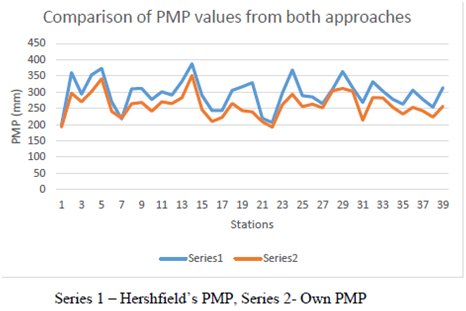
Where $PM{P}_{HMR}$ is the PMP values from the HMR documents. Using the PMP values and the mean and standard deviation of stations, the range of $k_m$ was from 22.2 to 26.6. It was too high with a narrow difference between the highest and lowest values. It is because the PMP values published in HMR are too high as compared to the average precipitation amount and the PMP estimated using basic-specific enveloping curve. This shows the significance of constructing the basin-specific enveloping curve for calculating PMP. PMP values were estimated for every duration and each station using both basin-specific curve and Hershfield’s curve. Figure 4 compares Hershfield’s PMP estimates against PMP estimates for Brazos River basin based on 1-hour duration. It was observed that for the 1-hour duration PMP values were 16.8% higher using Hershfield’s curve than using the basin-specific curve, 18.5% for 6-hour duration, and 23.4% for 24-hour duration which shows the uncertainty in the PMP estimates from the use of enveloping curve or using different values of it.

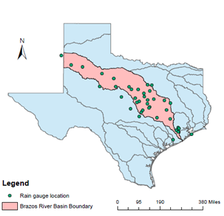
Figure 1 1-hour duration rain gauge station locations.

Figure 2 Enveloping curves of for different durations.Enveloping curves of for different durations.

Figure 3 Comparison of Hershfield’s enveloping curve of with Brazos River basin enveloping curve.
Series 1 – Basin-specific curve, Series 2- Hershfield curve

Figure 4 Comparison of Hershfield’s PMP estimates against PMP estimates for Brazos River basin based on 1-hour duration (mm).

Frequency analysis and Hazard rate

To quantify the uncertainty in PMP estimates, the best-fit probability distribution for the study area was determined. Using the same data of annual maximum precipitation, frequency analysis was performed using 24 alternative distributions that were Generalized Extreme Value distribution, Burr XII distribution, Dagum, Log-logistics (3 parameter), Pearson 5 (3 parameter), Generalized Gamma (4 parameter), Pearson 6 (4 parameter), Log-normal (3 parameter), Generalized Gamma (3 parameter), Burr (4 parameter), Fretchet (3 parameter), Pearson 6 (2 parameter), Generalized Beta of the second order (4 parameter), Gumbel max, Log-Pearson 3, Log Gamma, Johnson SB, Inverse Gaussian (3 parameter), Dagum (4 parameter), Inverse Gaussian (2 parameter), Log-logistics (2 parameter), Frechet (2 parameter), Pearson 5 (2 parameter), and Log-normal (2 parameter). Three goodness of fit (GOF) tests, Kolmogorov-Smirnov (K-S) test, Anderson-Darling (A-D) test, and Chi-square (C-S) test, were employed to check whether a hypothesized distribution function fitted the sample data (Chakravarti et al.,1967). The hypothesis for the GOF tests was: H0=The precipitation data followed the specific distribution; and H1=The precipitation data did not follow the specific distribution.

These tests were performed at the significance level (α=0.05) for choosing the best-fit probability distribution (Sharma and Singh, 2010). Q-Q plot and Root Mean Square Error (RMSE) were also used to find the best-fit probability distribution. Extreme precipitation data were fitted to all the distributions and parameters of the distributions were estimated by the maximum likelihood estimation and L-moments. The probability density functions (PDFs) were determined and plotted. Matlab and R-statistics were employed for fitting the probability distributions. A ranking system, based on the lowest test static value of GOF tests, was employed to determine the best-fit probability distribution. In the initial processing, all 24 common statistical distributions were used in this step. Some of the common distributions are shown in Table 1 along with their PDFs and CDFs. For each station and duration the test statistic values of Kolmogorov-Smirnov, Anderson Darling, and Chi-square were calculated for every distribution. For each of the three tests the distributions were ranked according to the lowest test statistic value. The distribution having the 1^st rank was assigned a score of 24, 2^nd rank distribution a score of 23, and so on. The total scores from the three tests of each distribution were added to see which distribution had the highest score, the second highest, and so on. At least 5 to 6 distributions were considered for further analysis. The stations were ranked according to the least RMSE value and best Q-Q plot (Here best means Q-Q plot is linear or the specified theoretical distribution is the correct model.). Sometimes the tests are also biased so it is helpful to see the PDFs of the distributions to see how well they fit the data at the right tail to make sure the results are consistent with the GOF tests or not. The PDFs of the selected 5 or 6 distributions were compared to see if our results were consistent with the PDF graph or not.

In the last step, for those stations and durations for which the difference in the PDF graphs of selected distributions was not too much or there were contradicting results by observing the quantiles of the distributions with the observed values against the MSE and Q-Q plot results, the ranking system was used again. The top 5 or 6 distributions from step 1 were selected. The distributions were ranked according to the test statistic value from the K-S, A-D, C-S, RMSE tests and visually seeing Q-Q plots. A score of 5 or 6 was assigned to the best distribution for a particular test and so on. The distribution having the highest combined score from the 5 tests was regarded as the best distribution. After the best distribution was selected, it was analyzed to see which distribution fitted most of the stations and for different durations overall. The Burr XII distribution was chosen to be the best distribution for the Brazos River basin covering 30 to 40% of the stations for different durations. For other stations also, it was, in most of the cases, one of the top three best distributions. Hazard rate is defined as the instantaneous rate of failure for the survivors to time t during the next instant of time. In flood frequency analysis it can be defined as the probability of extreme flooding in an infinitesimally small time period between t and t+dt given that no flooding has occurred until time t or the rate of event occurrence per unit of time. It is not a density or probability but a measure of risk. As greater the hazard between times t and t₁, greater is the risk of failure in this time interval. Hence, once the best-fit distribution was determined using different GOF tests it was seen how the hazard function varied with other distributions and durations to study more about the distribution, as it has more physical significance. As in case of agricultural lands, the hazard due to flooding will increase to a particular extent and then will become constant or can even decrease as the water will saturate to a certain limit and at that point no further damage would result, hence the hazard rate will tend to become constant. It was therefore decided to calculate the hazard rate for different distributions and durations to determine which distribution performed better. The hazard rate (h(t)) was calculated as²²

$h(t)=\frac{f(t)}{1-F(t)}$ (3)

where $f(t)$ is the probability density function or the probability that the value (failure or death) will fall in a specific interval and $F(t)$ is the cumulative distribution function. $1-F(t)$ can be defined as a survival function or the probability of surviving up to time t.

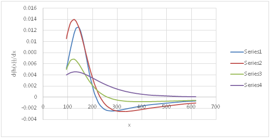
Based on equation (3), the hazard rate was calculated for different distributions and durations. For distributions with 2 parameters there was a general trend of increasing hazard rate. Figure 5 shows the hazard rate for 5 common distributions for 2-hour duration at station Flat. It is observed that Gumbel Max and Inverse Gaussian (2 parameter) had an increasing hazard rate which then tended to become constant, while the Burr XII and log-logistic (3 parameter) and GEV had an increasing hazard rate which then became constant and started decreasing. It makes sense physically, as station at Flat lies in Post Oak Belt in Texas where Prairie grasslands are scattered throughout the area, the damage rate due to flooding will increase to a certain extent and then will become constant and start decreasing. To determine how the hazard rate was changing, it was differentiated with respect to extreme precipitation x. Using the probability density function (PDF) and cumulative distribution function (CDF) of the distributions d(h(x))/dx was calculated. Figure 6 shows the rate of change of hazard rate for the same 2-hour duration at station Flat. The rate of change of hazard rate generally followed the same trend for all four distributions, except that the rate of change was non-negative for Gumbel distribution. It shows how quickly the hazard rate is increasing or decreasing with respect to extreme precipitation. To further study these characteristics it was also determined how hazard rate and rate of change of hazard rate varied in different climatic regions in Brazos River basin. There was no significant pattern, but it was observed that for stations near the Gulf there was an increasing hazard rate for most of the distributions. For stations away from the Gulf, the hazard rate followed the trend of increasing first, becoming constant and then decreasing. It can be due to the reason that the average annual rainfall decreases with increasing distance from the Gulf of Mexico (Singh and Hao, 2012).

Figure 5 Hazard rate for different distributions for 2-hour duration at station Flat.

Figure 6 Rate of change of hazard rate for different distributions for 2-hour duration at station Flat.
Series 1 – Burr, Series 2- Log logistics (3P), Series 3 – GEV, Series 4 – Gumbel max.

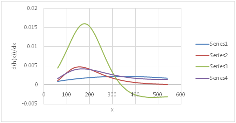
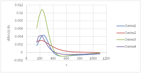
It may be noted that for stations close to the Gulf the histogram was smooth but had more variation. As the distance from the Gulf increased the histogram began to become sharp with less variation. Figure 7, Figure 8& Figure 9 show the hazard rate for different distributions at three stations, Lubbock (upstream), Coryell (middle), and Houston Addicts (downstream), for 24-hour precipitation. For higher durations of precipitation, the GEV distribution also began to reach a constant hazard rate. The rate of change of hazard rate was also calculated for the same distributions and durations. The log-logistic distribution consistently gave a higher rate of change and the Gumbel distribution gave a non-negative rate of change. Figure 10, Figure 11 & Figure 12 shows the rate of change of hazard rate for the same distributions and stations as above. The pattern varied across the study area but the Burr XII and GEV distributions performed better except in regions close to the High Plains division in which the maximum precipitation derives from thunderstorms during the summer season. Burr XII also performed better, based on different GOF tests as stated earlier.

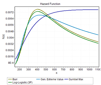
Figure 7 Hazard rate for different distributions for 24-hour duration at station Coryell.

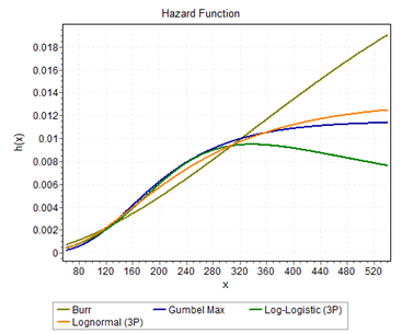
Figure 8 Hazard rate for different distributions for 24-hour duration at station Houston Alife.

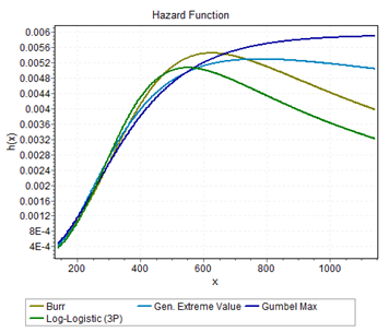
Figure 9 Hazard rate for different distributions for 24-hour duration at station Lubbock.

Figure 10 Rate of change of hazard rate for different distributions for 4-hour duration at station Houston Addicts.
Series 1 – Burr, Series 2 - Gumbel max, Series 3 – - Log logistic (3P), Series 4 – GEV

Figure 11 Rate of change of hazard rate for different distributions for 24-hour duration at station Coryell.
Series 1 – Burr, Series 2 - Gumbel max, Series 3 – - Log logistic (3P), Series 4 – GEV.

Figure 12 Rate of change of hazard rate for different distributions for 24-hour duration at station Lubbock.
Series 1 – Burr, Series 2 - Gumbel max, Series 3 – - Log logistic (3P), Series 4 – GEV.

Uncertainty in PMP estimates due to sample mean and sample standard deviation

To quantify the uncertainty of PMP due to sample mean and sample standard deviation, a procedure developed by Salas et al.,²³ was followed. To quantify the uncertainty required the calculation of variance ($Var(P)$ ) of PMP estimates which was calculated as^16,24

$Var(P)=Var(\overline{X_n})+k_m{}^{2}Var(S_n)+2k_{m}Cov(\overline{X_n},S_n)$ (4)

Where $Var(\overline{X_n})$ the variance of the mean is, $Var(S_n)$ is the variance of standard deviation and $Cov(\overline{X_n},S_n)$ is the covariance of mean and standard deviation. The requirement was to calculate $Var(S_n)$ and $Cov(\overline{X_n},S_n)$ . To calculate it,¹⁶ used Monte Carlo simulation experiments assuming Gumbel distribution (GEV-Type I) as the underlying distribution of the process under construction. Then, for easy application, the variance and covariance terms were determined based on the normal approximation, and a correction factor used for obtaining them for the Gumbel distribution. Furthermore, this study was extended by assuming the log-Gumbel (GEV-Type II) distribution.²³ However, for Brazos River basin using precipitation data the best fit distribution was Burr XII, hence, a different methodology was developed which would be suitable for the study area.

The values of first shape parameter, second shape parameter $\kappa$ and scale parameter$\beta$ of the Burr XII distribution were used along with Monte Carlo analysis. The value of the first shape parameter  was in the range of 3.5 to 6.5 and the value of the second shape parameter $\kappa$ was in the range of 0.5 to 1.5 with a few exceptions like for 24-hour extreme precipitation at Groesbeck the value was 3.16, and for 1-hour extreme precipitation at Jeweet the value was 3.33. But the value of scale parameter $\beta$ varied readily from 150 to 400 and was even around 500 in a few cases. The value of $\beta$ tended to increase for higher duration of extreme precipitation. 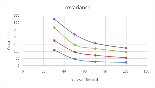Since the values of shape parameters had narrower ranges, the average values of $\alpha$ = 4.8 and $\kappa$ = 1 were used by taking the average of all the values. 1000 samples of different sizes n = 30, 50, 70, 100 and different scale parameter values of 150, 200, 300 and 400 were simulated and then the values of $\overline{X}(i)$ and $S_n(i)$ , i = 1,...,1000, were computed. $Var(S_n)$ and$Cov(\overline{X_n},S_n)$ were estimated, based on the pair of 1000 values, as shown in Table 2. It was observed that with increasing scale parameter $Var(S_n)$ and $Cov(\overline{X_n},S_n)$ increased, but decreased with increasing record length (n). It can be expected because by increasing the scale parameter the spread increases, hence that leads to a larger variance.

To check whether the values of $\alpha$ = 4.8 and $\kappa$ = 1 would give reliable results, simulations were also run for the shape parameter values $\alpha$ = 5.3 and $\kappa$ = 0.8. These values were the average values for 24 hour duration extreme precipitation. The scale parameter value of 150 for the first simulation and 300 for the second simulation were used. It was because 150 was the least scale parameter value and 300 was the average value for 24 hour duration extreme precipitation series. The results for different record lengths of 30, 50, 70, and 100 years were not very different from the one using the values of $\alpha$ = 4.8 and $\kappa$ = 1, as shown in Table 3. Hence, it was decided to use the values of $\alpha$ = 4.8 and $\kappa$ = 1 as the average values for calculating $Var(S_n)$ and $Cov(\overline{X_n},S_n)$ . Then, a nomograph of varying scale parameter $\beta$ and varying record length was constructed, as shown in Figure 13 & Figure 14. From these figures the values of $Var(S_n)$ and $Cov(\overline{X_n},S_n)$ were determined for all the stations with different durations having the Burr XII distribution as the best distribution. Then, $Var(P)$ was determined based on equation (4).

As in Salas et al.,¹⁶ the expected value of PMP estimate $E(P)$ was calculated as:

$E(P)=E(\overline{X_n})+k_{m}E(S_n)$ (5)

Where$E(\overline{X_n})$ is the expected value of the sample mean and $E(S_n)$ is the expected value of the sample standard deviation. It can be shown²⁴ that:

$E(\overline{X_n})=E[\frac{1}{n}{\displaystyle \sum _{i=1}^n{X}_i}]=\frac{1}{n}{\displaystyle \sum _{i=1}^{n}E(X_i)=\mu }$ (6)

and

$E(S_n)=\frac{\Psi (n/2)}{\Psi [(n-1)/2]\sqrt{(n-1)/2}}\sigma$ (7)

Where$\mu$ and $\sigma$ are the population mean and standard deviation, $\Psi (a)$ is the incomplete gamma function with argument a, and n is the record length. Using equations (6) and (7) the expected value of PMP value was calculated as:

$E(P)=\mu +\frac{\Psi (n/2)}{\Psi (n-1)/2\sqrt{(n-1)/2}}\sigma$ (8)

Where$\mu$ and $\sigma$ are the population mean and standard deviation which were replaced by the corresponding sample estimates after appropriate adjustments for outliers as needed. $\Psi (a)$ is the incomplete gamma function defined as:

${\displaystyle \underset{0}{\overset{\infty }{\int }}{t}^{a-1}{e}^{-t}dt}$ (9)

Where a is the argument. Following Salas et al.,¹⁶ the design risk PMP value $P_d$ was calculated as:

$P_d=E(P)\pm c\sigma (\stackrel{}{P)}$ (10)

Where$\sigma (\stackrel{}{P)}$ is the standard deviation of PMP estimates, and c>1 is the parameter. $P_d$ is the value of uncertain PMP value P whose distribution is not known but only the estimates of its mean $E(P)$ and standard deviation $\sigma (\stackrel{}{P)}$ are known. Table 4 compares 1-hour PMP values at Thompson, Texas, obtained using the statistical method and the method considering the Burr XII distribution for calculating $Var(S_n)$ and $Cov(\overline{X_n},S_n)$ . At Thompson, for 1-hour duration of extreme rainfall the value of adjusted $X$ and $S_n$ was 50.28 mm and 22.18mm. The value of $k_m$ obtained from the enveloping curve was 7.86. The best-fit distribution at the station was the Burr XII distribution with scale parameter $\beta$ =165.43 and record length (n) = 52. From Figure 6 & Figure 7, the values of $Var(S_n)$ and $Cov(\overline{X_n},S_n)$ were obtained as 190 and 50. Using equations (8) and (9) and $Var(P)$ were 223.29 mm and 3218.1 mm, respectively, and $\sigma (\stackrel{}{P)}$ was calculated by taking the square root of $Var(P)$ . For different values of c the design risk PMP $P_d$ was calculated. With c = 1 and +sign $P_d=E(P)+c\sigma (P)$ gave = 251.88mm. The value of c = 3 which was a more conservative estimate than using c=1 which gave $P_d$ 309.06mm. Using Hershfield’s original method along with basin-specific enveloping curve the PMP estimate P was 253.45mm after multiplying the PMP value with 1.13 for fixed observational time interval. The PMP values were also calculated using the Salas et al.,¹⁶ method. It gave a PMP value of 241.2mm and using normal distribution and it gave a PMP value of 231.65mm. Results showed some differences between PMP values using all the three methods. It can be concluded that a bigger value of PMP must be selected, considering the associated exceedance probabilities (risk). The analysis was performed for other durations and stations having the Burr XII distribution as the best distribution. Table 5 shows the 24-hour design risk values for different values of c. As in Salas et al.¹⁶ Chebyshev’s inequality²⁵ was used to have a bound of the probability on PMP estimates based in equation (7):

$P\{(E(P)-c\sigma (P)<PMP<E(P)+c\sigma (P)\}\ge 1-\frac{1}{c^2}$ (11)

Using the same data for 1-hour PMP values at Thompson, Texas, it can be shown that:

 For c = 1 $P\{194.70<P<251.88\}\ge 0.0$

 For c = 2 $P\{166.11<P<280.47\}\ge 0.75$

 For c = 3 $P\{137.52<P<309.06\}\ge 0.89$

Figure 13 N=57; Epidemiological distribution of the pathological fractures, traumatic fractures, and nonunion.
Series 1: = 150, Series 2: = 200, Series 3: = 300, Series 4: = 400

Figure 14 Covariance of mean and standard deviation as a function of record length.
Series 1: = 150, Series 2: = 200, Series 3: = 300, Series 4: = 400

It shows that there is less than 11% probability that the PMP estimate P is bigger than 309.06mm and smaller than 137.52 for c=3. The probability bound suggested that the value of 251.88 mm had a higher chance to be exceeded because of the uncertainty associated with the estimates of $X$ , $S_n$ and record length of 52. The value of 309.06 mm corresponded to a more conservative estimate that was less likely to be exceeded because of the uncertainty associated with $X$ and $S_n$ . It took into account the effect of uncertainty and the associated probability of exceedance.

Uncertainty in PMP estimates using first order second moment analysis

The first order second moment (FOSM) analysis was used to determine the uncertainty introduced in the PMP estimates due to various parameters. Let PMP be a function of mean, standard deviation and frequency factor. Then,

$PMP=g(x)$ , $x:(x_1,x_2,x_3)$

Then, in terms of PMP formula, $g(x)$ can be expressed as:

$g(x)=x_1+x_2\times x_3$ (12)

Where $x_1$ =The mean of PMP estimates, $x_2$ =The standard deviation of PMP estimates, and $x_3$ =The frequency factor of PMP estimates.

From Taylor series expansion up to second orders about the mean it can be shown that:

$g(x)=g(\overline{x)}+(x-\overline{x)}\frac{dg(x)}{dx}+\frac{(x-{\overline{x)}}^2}{2}\frac{d^{2}g(x)}{d{x}^2}$ (13)

Taking the first order approximation the expected value of PMP estimates were determined, based on²⁶

$E(PMP)=g(\overline{x)}$

where $\overline{x}=(\overline{x_1},\overline{x_2},\overline{x_3})$ and $x$ is the mean value of mean of PMP estimates, $x_2$ is the mean value of standard deviation, and $x_3$ is the mean value of frequency factor. The variance of PMP due to each random component around the mean was calculated as:

$Var(PMP)={{\displaystyle \sum _{i=1}^{i=k}(\frac{dg(x)}{d{x}_i})}}^2{\sigma }_i{}^2$ (14)

Where, x_i, i = 1…k, are random variables and ${\sigma }_i$ is the standard deviation of each component.

The expected value of PMP estimates for 1-hour duration was 276mm with the standard deviation of 32mm due to mean, 22mm due to frequency factor, and 16 mm due to standard deviation. For the 6-hour duration the expected value was 346mm with the standard deviation of 39mm due to mean, 26.2mm due to frequency factor, and 17.9mm due to standard deviation. For 24-hour duration the expected value was 423mm with the standard deviation of 45.3 due to mean, 29.4mm due to frequency factor, and 21.4mm due to standard deviation. To determine the relative contribution of each random component to the total uncertainty of PMP, the coefficient of variation was calculated as:

$Cov=\frac{{\sigma }_i{}^2}{{\mu }_i{}^2}={{\displaystyle \sum _{i=1}^{i=k}(\frac{dg(x)}{d{x}_i})}}^2\frac{{\sigma }_i{}^2}{{\mu }_i{}^{2^{}}}$ (15)

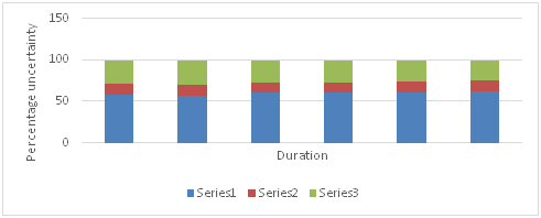
Where the term ${(\frac{dg(x)}{d{x}_i})}^2{\sigma }_i{}^2$ of each random component was calculated for the total uncertainty of PMP estimates. It was observed that for 1-hour duration 58% uncertainty was introduced due to mean, 27% due to frequency factor and 14% due to standard deviation. For 6 hour duration the uncertainty was 60.4% due to mean, 27.2% due to frequency factor and 12.5% due to standard deviation. For 24-hour it was 60.95% due to mean, 25.5% due to frequency factor and 13.5% due to standard deviation. Figure 15 shows the relative contribution of each component to uncertainty for different durations of 1, 2, 3, 6, 12 and 24 hours. It can be observed that the relative contribution to uncertainty for different durations was almost the same with the maximum uncertainty introduced due to the mean of annual maximum precipitation series.

Figure 15 Relative uncertainty of each component to the total uncertainty in PMP estimates.
Series 1- Mean, Series 2 – Standard deviation, Series 3- Frequency factor

Data collection and manipulation for Risk analysis of extreme precipitation

The flood damage data for Harris County was requested from FEMA which maintains the National Flood Insurance Program (NFIP). The data comprised the flood event, amount of damage in dollars for a particular flood event on a particular area which was characterized by 5 digit zip codes, the date of the event and the amount paid by NFIP. The flood events were from the period of year 1978 to 2002. In the Harris County there were two rain gauges Houston Alife and Houston Addicts. For gathering precipitation events at the two stations associated with the flood event hourly precipitation data from NCDC NOAA was used. To account for the effect of wet catchment before a storm, antecedent precipitation index (API) was used. Wet catchment and heavy rain can lead to flooding. API was calculated as²⁷

$AP{I}_n=P_n+k{P}_{n-1}+k^2{P}_{n-2}+\mathrm{...}$ (16)

Where $AP{I}_n$ is the Antecedent Precipitation Index for day n,k is the empirical decay factor less than one, and $P_n$ is the precipitation for day n. The catchment wetness decline each day by the factor k. API goes up again by any rain. A value of 0.90 was used for k.⁴

Precipitation events associated with the flood date were selected. Point rainfall estimates (rainfall depth reading at the station) covers an area of 25×25km² area and rainfall events which occurred at those stations were taken. There were other stations in the county but it was seen from the precipitation database and storm record that only those events which had storm center across the location were taken. It may be noted that two precipitation events were considered independent when there was a certain dry period in between without or with minor precipitation. Urban drainage systems have a lagged response to precipitation and need a certain time to restore the equilibrium state. The flood damage can be completely related to a particular precipitation event if systems are in equilibrium state before a precipitation event. A typical time for sewer systems to restore equilibrium state is between 10 and 20hours.²⁰ hence, the precipitation events were selected that had at least 10- to 12-hour time difference between them. Also, the precipitation amount less than 1 mm/hour was treated as no precipitation. That prevented unrealistic long precipitation events to exist because of very small precipitation amounts between precipitation events. The damage amounts in (US) dollars for the flood events were arranged and adjusted for Consumer Price Index Inflation.²⁸ The damage data was given for zip areas in Harris County; hence, for calculating the total damage due to a precipitation event the damages in all the zip areas up to which the event extended were added. As a point rainfall estimate is applicable to a 25×25km area, the zip areas which covered that area were also used for damage analysis. A weighted average function was developed, depending upon the amount of precipitation for the rain gauges, the duration of precipitation and the closeness of zip area to the rain gauge. The total damage values were distributed among the zip areas for precipitation events occurring at both the stations and were added to have the total damage due to a particular precipitation event.

Estimation of risk and assessment of damage

The exceedance probabilities were calculated for precipitation events associated with flood events from frequency analysis. The expected loss or risk associated with a precipitation event was calculated as (11):

$E\left(L\right)=p_i\times L_i$ (17)

Where E_i is the expected loss for a given event, p_i is the probability of exceedance of a precipitation event, and L_i is the associated loss.

Table 6 shows the exceedance probabilities of precipitation events, total damage and the expected loss or the associated risk in a given year for Houston Alife station. As can be seen, the expected loss due to precipitation events was very high. Due to the limitation of data, there were not many precipitation events of different durations so that the probability of exceedance can be correlated with damage amount. The exceedance probability was plotted against the total damage for 12-hour flood events at Houston Addicts station and 6-hour flood events at Houston Alife station. Figure 16 & Figure 17 show the correlation curves for both stations along with the fitted regression equation. The exceedance probability of PMP was fitted to the equations for both stations. Table 7 shows the exceedance probability of PMP value and total damage. As can be seen, the total damage amount is very high. The damage due to a single PMP event of 12-hour duration can be as high as 2 billion dollars. It shows how much damage a single PMP event can cause. It may be noted that more events would have given better results.^29‒32

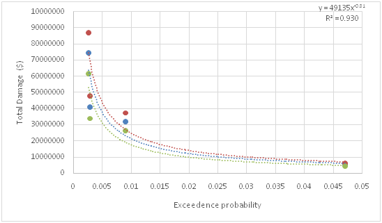
Figure 16 Correlation curve between exceedance probability of PMP and total damage for 12 hour duration precipitation at Houston Alife.

Figure 17 Correlation curve between exceedance probability of PMP and total damage for 6 hour duration precipitation at Houston Addicts.

It can be seen from this study that large uncertainty can be introduced in the PMP estimates due to the uncertainty in sample mean, standard deviation, and frequency factor values. The Burr XII distribution came out to be the best-fit distribution using frequency analysis of extreme rainfall and hazard rate. Using the parameters values of Burr XII distribution and Chebyshev’s inequality, probability bounds on the PMP estimates were calculated which suggested that the value of PMP had a higher chance to be exceeded because of the uncertainty associated with the estimates of sample mean, sample standard deviation and frequency factor. The PMP values were also calculated using Gumbel distribution and normal distribution and it came out to be lower than the proposed method. The relative contribution of each component was also calculated and it was observed that uncertainty was higher due to mean than standard deviation and frequency factor. The expected loss for extreme precipitation events was determined and exceedance probabilities of extreme precipitation events were correlated with the associated total damage. It was found that the total damage a single PMP event of 12-hour duration can cause can be as high as 2 billion dollars in Harris County, Texas.

This study was supported in part by the project “Quantifying Uncertainty of Probable Maximum Flood (PMF),” contract No. DOD-USACE contract W912HZ-16-C-0027, funded by US Army Engineer-Engineer Research Development Center, Vicksburg, Mississippi.

The author declare there is no conflict of interest.

1. US National Weather Service. Probable Maximum Precipitation–United States between the Continental Divide and the 103rd Meridian. Hydrometeorological Report No. 55A (HMR-55A), Silver Spring, MD, USA. 1988;1‒51.
2. Schreiner LC, Riedel JT. Probable Maximum Precipitation Estimates. United States East of the 105th Meridian HMR No. 51. National Weather Service, National Oceanic and Atmospheric Administration, United States Department of Commerce, Washington, DC. 1978.
3. Tomlinson EM, Kappel WD. Dam Safety: Revisiting PMPs. Hydroworld.com, Tulsa, Okla. 2009.
4. US Department of Commerce. Generalized Estimates of Probable Maximum Precipitation for the United States West of the 105thMeridain. Technical Paper number 38. 1960;1‒82.
5. Kulkarni BD. Generalized Physical Approach of Estimating Areal Probable Maximum Precipitation for Plain Region of the Godavari River Basin (India). Journal of Spatial Hydrology. 2010;2(2).
6. Chow VT. A General Formula for Hydrologic Frequency Analysis. Transactions- American Geophysical Union. 1951;32:231‒237.
7. World Meteorological Organization. Manuel on Estimation of Probable Maximum Precipitation. WMO-No 1045, Geneva, Switzerland. 2009.
8. Casas MC, Rodriguez R, Nieto, R, et al. The Estimation of Probable Maximum Precipitation: The Case of Catolonia. Annals of the New York Academy of Sciences. 2008;1146:291–302.
9. Hershfield DM. Method for Estimating Probable Maximum Rainfall. American Water Works Association. 1965;57(8):965‒972.
10. Koutsoyiannis D. A Probabilistic view Of Hershfield’s method for Estimating Probable Maximum Precipitation. Water Resources Research. 1999;35(4):1313‒1322.
11. Hershfield DM. Estimating the Probable Maximum Precipitation. Journal of Hydraulics Division. 1961;87(5):99‒106.
12. Srinivas VV, Chavan SR. Probable Maximum Precipitation Estimation for Catchments in Mahanadi River Basin. Aquatic Procedia. 2015;4:892–899.
13. Micovic Z, Schaefer MG, Taylor GH. Uncertainty Analysis for Probable Maximum Precipitation Estimates. Journal of Hydrology. 2014;521(2015):360‒373.
14. Koutsoyiannis D, Papalexiou SS. A probabilistic approach to the concept of Probable Maximum Precipitation. Advances in Geosciences. 2006;7:51‒54.
15. NRC (National Research Council). Risk Analysis and Uncertainty in Flood Damage Reduction Studies. National Academy Press, Washington DC; 2000;202.
16. Salas JD, Gavilan G, Salas FR, et al. Uncertainty of the PMP and PMF. Chapter 28, Handbook of Engineering Hydrology, Vol.2, In: Eslamian S, editor. Modeling, Climate Changes and Variability. Taylor & Francis, CRC Press. 2014.
17. Koks EE, Moel H, Koomen E. Comparing Extreme Precipitation and Large-Scale Flooding Induced Inundation Risk– Evidence from a Dutch Case-Stud. VU University Amsterdam, Nederland’s. 2012;1‒25.
18. Villalta DE, Guenni B, Sajo-Castelli AM, et al. Risk analysis to extreme precipitation: A retrospective approach. Presentation. PASI. 2014;1‒44.
19. Kunreuther H, Meyer R, Bulte CVD. Risk Analysis for Extreme Events: Economic Incentives for Reducing Future Losses. National Institute of Standards and Technology, Gaithersburg. 2004.
20. Spekkers MH, Kok M, Clemens FHLR, et al. A statistical Analysis of Insurance Damage Claims Related to Precipitation Extremes. Hydrol Earth Syst Sci. 2012;17:913–922.
21. David SA, Skaggs LL. Catalog of Residential Depth-Damage Functions used by the Army Corps of Engineers in Flood Damage Estimates. U.S Army Corps of Engineers. IWR Report 92-R-3. 1992.
22. Read LK, Vogel RM. Hazard Function Analysis for Flood Planning under Nonstationarity. Water Resources Research. 2016;52.
23. Salas JD, Salas FR. Estimating the uncertainty of the PMP. Paper presented to the XXVII IAHR Latinamerican Congress of Hydraulics. 2016.
24. Kendall M, Stuart A. The Advanced Theory of Statistics. Distribution Theory, New York; Hafner Publishing Company, Inc. 1963.
25. Mood A, Graybill F, Boes DC. Introduction to the Theory of Statistics. 3rd edition. New York; McGraw Hill. 1974.
26. Ang AHS, Tang WH. Probability Concepts in Engineering Planning and Design. Basic Principles, New York; John Wiley. 1975.
27. Ball J, Babister M, Nathan R, et al. Australian Precipitation and Runoff: A Guide to Flood Estimation. Commonwealth of Australia (Geoscience Australia). 2016.
28. Smith AB, Matthews JL. Quantifying Uncertainty and variable sensitivity within the US billion-dollar Weather and Climate Disaster Cost Estimates. Nat Hazards. 2015;77(3):1829‒51.
29. Koutsoyiannis D. Statistics of Extremes and Estimation of Extreme Precipitation II: Empirical Investigation of Long Precipitation Records. Hydrological Sciences Journal. 2004;49(4):591–610.
30. Kousky C, Kerjan EM. Examining Flood Insurance Claims in the United States: Six Key Findings. The Journal of Risk and Insurance. 2015;84(3):819‒850.
31. Willeke GE. Myths and uses of Hydrometeorology in Forecasting. Proceedings of March 1979 Engineering Foundation Conference on Improved Hydrological Forecasting- Why and How. American Society of Civil Engineers, New York. 1980;117‒124.
32. World Meteorological Organization. Manual for Estimation of Probable Maximum Precipitation. Operational Hydrology Report1, 2nd edition, Publication 332, World Meteorological Organization, Geneva. 1986.