This study is all about rainfall intensity – duration - frequency (IDF) modeling based on probability and non-probability distribution function (PDF, and nPDF). A set of sixteen year rainfall amounts and durations for Port Harcourt metropolis was adopted for the modeling. The study involved the application of the following distribution functions: Gumbel Extreme Value Type-1 (Gumbel EVT-1), Normal, Pearson Type-3 (PT-3), Log Pearson Type-3(LPT-3), and Log-Normal (L-N), respectively. And the nPDF in the form of Talbot simple quotient, power, and Sherman quotient-power models. To implement the PDF modeling it was necessary to generate frequency factors for each of the five models. This was followed by non-linear regression analysis which involved the use of Excel Solver with optimization technique in Microsoft Excel applied to estimate the parameters of the IDF models. All the PDF-IDF models were calibrated using the Sherman’s equation as general models for which the intensity value is a function of return period and rainfall duration. A comparative analysis was carried out between PDF and nPDF IDF models predicted intensities that showed a good match with observed intensities. The Normal distribution IDF model ranked the best with respect to mean squared error (MSE=92.71) and goodness of fit (R²=0.970) in PDF model category, while Gumbel EVT-1 model was second best (MSE=109.39, R²=0.975), and showed better result on each of the specified return period (2, 5, 8 and 16 years). In all, no significant difference amongst the predicted intensities of the various IDF models (PDF and nPDF models).

Keywords: probability and non-probability distribution functions, rainfall intensity, duration, modeling, port harcourt

Flooding incidence has caused damage to properties and loss of human lives in urban centers in Nigeria and elsewhere and have since increased tremendously.^1,2 It is very important to have measures to help estimate rainfall intensity more accurately because prolonged and intense heavy rainfall has been known to contribute more to flooding menace. Especially now that issues of climatic change seems to make worse and create uncertainties in estimating rainfall records for flood analysis needed for planning and design of storm water management facilities. The essential instrument required for deriving the characteristics of rainfall in any catchment area is a Rainfall Intensity- Duration-Frequency (IDF) model. The rainfall models are developed usually from a long time rainfall records for a given weather station, and these are seriously inadequate or lacking in most developing countries.

Early scholars who have made contributions in IDF modeling include Meyer,³ Sherman,⁴ Bernard⁵ and Bilham.⁶ The developed equations were valid for durations between 5 and 120 minutes. Bilham⁶ equations overestimated the probabilities of high intensity rainfall in the United Kingdom. Holland⁷ updated and made easier the Bilham equation and extended the duration to 25hrs. Hershfield⁸ provided different isohyetal maps that estimated design rain depths of various specified durations and corresponding return periods for given regions in USA. Bell⁹ generalized the formula by deriving an IDF model which enabled the computation of depth-duration as an index for certain locations in USA. Chen¹⁰ also derived applicable IDF curves for the USA. Mathematical methods have been proposed to model extreme storm probabilities taken from the scaling properties of data observed in a station rainfall records. Bara et al.¹¹ worked on method of deriving IDF curves of extreme rainfall events by applying simple scaling theory to the characteristics of the IDF of rainfall with short durations in Slovakia. On the other hand, AlHassoun¹² developed empirical formulae for calculating rainfall intensity in the region of Riyadh. He opined that there was no significant difference in the results of the curves of the IDF models obtained in Riyadh area between the Log-Pearson Type-3 (LPT-3) and Gumbel EVT-1 methods. He concluded that the semi-arid climate with flat topography of the region must have accounted for the results. Elsebaie,¹³ also worked in Saudi Arabia and obtained results that were very similar to that of Riyadh study using the Gumbel EVT-1 and LPT-3.

In Nigeria, the development of IDF models is still in its growth path and is limited to the extent of available data. Oyebande¹⁴ derived rainfall IDF model for the western regions without adequate data. He applied the Gumbel EVT-1 distribution to the maximum period of ten year records available to derive rainfall IDF models. Recent research works on IDF development are those of Nwaogazie & Duru¹⁵ for Port Harcourt city. Nwaogazie & Uba¹⁶ for Eket city; and Nwaogazie & Ologhadien¹⁷ for Southern Nigeria, Okonkwo & Mbajiorgu¹⁸ for South Eastern Nigeria. The IDF curves developed were in accord with IDF theory for shorter recurrence periods of 2 to 10 years. Akpan & Okoro¹⁹ developed IDF for Calabar; and Akpen et al.²⁰ studied for Makurdi metropolis. However, a recent study published by Nwaogazie & Okonkwo²¹ on comparative analysis of four types of IDF models developed for Abakiliki showed that only the simple quotient 2-parameter IDF model predicted the highest intensity values at short duration while the four models compared predicted approximately same intensities at higher durations. The aim of this study is to develop a Probability Distribution Function (PDF)-IDF models or PDF-IDF models for Port Harcourt metropolis using available rainfall intensities data with respect to the probability distribution functions (PDF) that best fit such observed data. This type of approach in IDF modeling had not been carried out for the study area.

Study area

The area of the study lies on latitude 4.46^o N and longitude 7.2^o E., (Figure 1). The study area is Port Harcourt metropolis and it stretches from Port Harcourt City through Obio-Akpor to Ikwerre Local Government Areas in Rivers State. The area experiences heavy seasonal rainfall between March and October with a dry period that last from November to February producing occasional rainfall. The climate is influenced by two air masses namely; the South Westerly wind from the Atlantic Ocean and the North East Trade wind from the Sahara desert. The area has a flat topography with inadequate drainage facilities and its elevation varies about 3 to 15m above mean sea level.²²

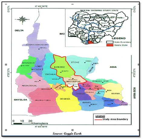
Figure 1 Location map of Study Area-Port Harcourt metropolis, Rivers State, Nigeria.

Data collection

The recorded daily rainfall data of Port Harcourt was obtained from Nigeria Metrological Agency (NIMET) Oshodi Lagos. The rainfall data obtained provided the amount of precipitation and the duration for sixteen year period, this showed rainfall events from the year 1998 – 2013. The annual maximum rainfall amounts were sorted out into durations of 10, 20, 30, 40, 50, 60, 90 and 120 minutes for each year of the sixteen years rainfall data. Thereafter, the rainfall data were ranked in decreasing order of their magnitude before selecting the peak rainfall for each year.

Data analysis

These sorted observed annual maximum rainfall amounts were further divided by the corresponding durations in hours to obtain the rainfall intensities (mm/hr) which were ranked in descending order of magnitude as shown in Table 1. Similarly the log-equivalent was computed including their statistical parameters (mean, standard deviation and coefficient of skewness). The California formula (see Equation 1) was used in computing the return periods for the non-probability distribution function (nPDF) IDF models.

$T_r=\frac{n}{m}$                                                                                  (1)

Where T_r = return period (years), m = rank order and n = total number of observations

Probability distribution function (PDF)-IDF models: The development of IDF relationship was achieved using probability distribution functions. The maximum rainfall intensity was computed for each of the commonly used probability distribution function (PDF) which is – Gumbel Extreme Value Type-1 (Gumbel EVT-1), Normal, Pearson Type-3 (PT-3), Log-Pearson Type-3 (LPT-3) and Log-Normal (LN) distributions. The approximation of the magnitude of a random event such as rainfall intensity is given in Equation (2) by Chow (1951) as:

$X_T=\overline{X}+ K_{T}S$        (2)

Where $\overline{X}$ = mean, S= standard deviation of the sample and $K_T$ = frequency factor. The last two parameters are functions of the return period, T and the PDF type. The determination of the value of rainfall intensity requires the computation of the frequency factor for each PDF, the mean and standard deviation for the observed data are substituted into Equation (2) for evaluation. Thus for:

1. Gumbel EVT-1 distribution - The $K_T$ was calculated using Equation (3).

$K_T= \frac{\sqrt{6}}{\pi }\left[0.5772+In\left[In\left[\frac{T}{T-1}\right]\right]\right]$           (3)

Where T = return period (years)

2. Normal Distribution- The $K_T$ was computed using Equations (4) and (5):

$K_T= Z= W-\frac{2.515517+0.802853\text{w}+0.010328{\text{w}}^2}{1+1.432788\text{w}+0.189269{\text{w}}^2+0.001308{\text{w}}^3}$                                (4)

Where $W={\left[In\left(\frac{1}{P^2}\right)\right]}^{\raisebox{1ex}{$1$}\!\left/ \!\raisebox{-1ex}{$2$}\right.}$ for (0 < p ≤ 0.5)                                                                                                               (5)

$p= \frac{1}{T}$ = probability function, and z = standard normal variate

3. Pearson Type-3 (PT-3) Distribution - The $K_T$ can be obtained from standard frequency factor table well published in literature or using Kite (1977) approximate method in Equation (6).

$K_T=Z+(z^2-1)k+1/3(z^3-6z)k^2-(z^2-1)k^3+z{k}^4+1/3k^5$          (6)

Where $k= \frac{C_s}{6}$ for $C_s\ne 0$ , but at $C_s=0$ , $K_T=Z$ . The $K_T$ can be seen to be dependent on the coefficient of skewness, $C_s$

4. Log-Pearson Type-3 (LPT-3) Distribution - The $K_T$ for LPT-3 was computed using same procedure as applied to PT-3 except that the mean, standard deviation and coefficient of skewness were obtained from logarithmically transformed data. Also, to compute the rainfall intensity value Chow²³ gave a logarithmically transformed version of Equation (2) reproduced here as Equation (7).

$\log X_T=\log \overline{X}+ K_T\log S$               (7)

5. Log-Normal Distribution- The rainfall values are also those converted to logarithmic form including the statistical parameters ($\overline{X}$ , S and $C_s$ ). Thevalues are obtained from Equations (4) and (5), while the magnitude of the rainfall intensities were computed from Equation (7).

Derivation of probability and non-probability IDF Equations: The Sherman modified quotient-power equation given by Chow et al.²⁴ and Raghumath²⁵ given as Equation (8) was adopted for the derivation of the IDF model.

Other IDF equations considered in this study are those of Equations (9) and (10). We note that only Equation (8) is dimensionless (unit less).

Sherman equation, $I=\frac{c{T}^m}{t^a}$                                 (8)

Talbot equation, $I=\frac{c}{b+t}$                                                          (9)

Power equation, $I=c{t}^a$                                                                   (10)

Where I=rainfall Intensity (mm/hr), t=duration (minutes) and T=return period (years); c, m, a and b are regional constants of the catchment area.

The calibrations of the IDF equations were achieved through the application of non-linear regression analysis. This method requires the use of Excel Solver which is an optimization technique in Microsoft Excel applied to estimate the parameters of IDF models.²⁶ The procedure requires feeding into the spreadsheet, PDF computed intensities as observed intensity values with their durations and return periods. Intensities corresponding to each duration and return period were calculated using the IDF equation such as Equation (8, 9 or 10) based on the assumed values of parameters of IDF equation. To obtain the values of optimum IDF parameters sum of square of deviation/error between observed intensity and predicted intensity were set to minimization using Generalized Reduced Gradient (GRG) solver as in Equation (11), thus the objective function becomes:

$MinSSE={\displaystyle \sum }_{i=1}^n{\left(I_{obs}- I_{pred}\right)}^2$                 (11)

Where $I_{obs}$ = observed or computed rainfall intensity, $I_{pred}$ = IDF model predicted rainfall intensity

n=number of data sets and i=an index (counter)

Solving Equation (11) produces the optimum values for the constants c, m, a and b achieved through iterative process that produces the least squared error. Further, Spiegel²⁷ and Zakwan²⁶ provided programmable formulas to obtain the coefficient of determination (R²) and the mean squared error (MSE) as in Equations (12) and (13):

$R^2=\frac{{{\displaystyle \sum }}_{i=1}^n{\left(I_{obs}- I_{avg}\right)}^2- {{\displaystyle \sum }}_{i=1}^n{\left(I_{obs}- I_{pred}\right)}^2}{{{\displaystyle \sum }}_{i=1}^n{\left(I_{obs}- I_{avg}\right)}^2}$                   (12)

$MSE= \frac{1}{n} {\displaystyle \sum }_{i=1}^n{\left(I_{obs}- I_{pred}\right)}^2$                                              (13)

Where $I_{avg}$ = average of observed or computed PDF rainfall intensity.

Similarly, the Easy-Fit Software was used to determine the goodness of fit statistic of the distribution models for this study on the observed rainfall intensity data. The software can be downloaded from (http://mathwave.com/easyfit-distribution-fitting.html)

Results

The result of the rainfall analysis of the sorted observed rainfall records for Port Harcourt metropolis are presented in Table 1 with the log equivalent. Included in the table are the statistical parameters (mean, standard deviation and coefficient of skewness) for each of the data set. Table 2 shows the summary of the distribution factors for Gumbel EVT-1 and Normal distribution factors computed. However the derived general IDF equations for each of the PDFs are shown in Table 3 alongside the corresponding goodness of fit (R²) and mean squared error (MSE) values. Figures 2-6 are the computed rainfall intensity values for Gumbel EVT-1, Normal, Log-Normal, Log-Pearson Type-3 and Pearson Type-3 distributions, respectively. Figure 7 & Figure 8 are graphical plots of PDF-computed intensities versus general PDF-IDF predicted intensities for Log-Pearson Type-3 and Gumbel EVT-1 which were best and worst fit distributions of the rainfall data, respectively. Table 4 & Table 5 show the summaries of three nPDF–IDF and three selected PDF–IDF calibrated models, in addition to goodness of fit (R²) and mean square errors, respectively. For sake of comparison, the results of calibrated nPDF-IDF models, and PDF-IDF models developed for specified return periods are shown in Figures 9 - 12 for 2, 5, 8 and 16 year return periods, respectively. The rainfall intensity data of Table 1 were subjected to normality test and the result confirmed not normal. Accordingly, Kruskal-Wallis Non-Parametric Analysis of Variance (ANOVA) was carried out for nPDF-IDF and PDF-IDF models for two segments of rainfall durations, that is, 10 – 40 minutes and 50 – 120 minutes, respectively to establish any significant difference or not (Table 6).

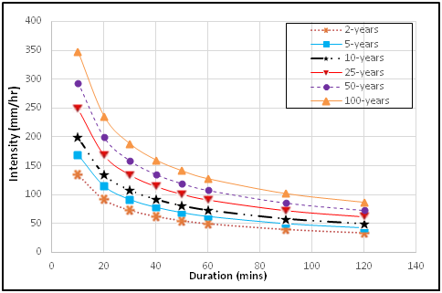
Figure 2 PDF-IDF curves for intensities of rainfall predicted from Gumbel EVT-1 IDF general model.

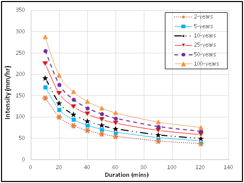
Figure 3 PDF-IDF curves for intensities of rainfall predicted from Normal IDF general model.

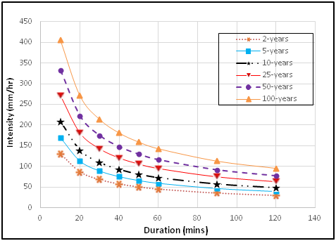
Figure 4 PDF-IDF curves for intensities of rainfall predicted from Log-Normal IDF general model.

Figure 5 PDF-IDF curves for intensities of rainfall predicted from Log-Pearson Type-3 IDF general model.

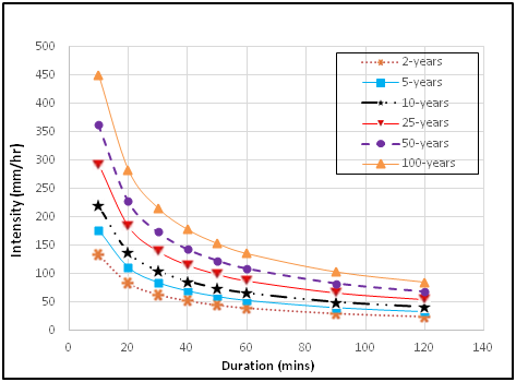
Figure 6 PDF-IDF curves for intensities of rainfall predicted from Pearson Type-3 IDF general model.

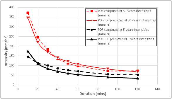
Figure 7 Log-Pearson Type-3 PDF-IDF curves for 5 and 50 years return period.

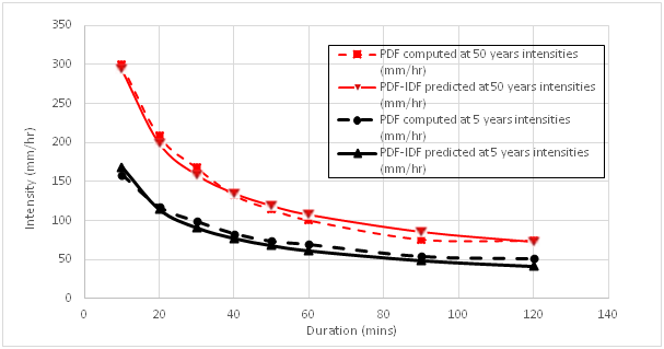
Figure 8 Gumbel EVT-1 PDF-IDF curves for 5 and 50 years return period.

Figure 9 Distribution of nPDF and PDF-IDF curves for Port Harcourt metropolis for 2 year return period.

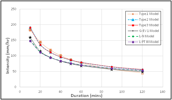
Figure 10 Distribution of nPDF and PDF IDF curves for Port Harcourt metropolis for 5 year return period.

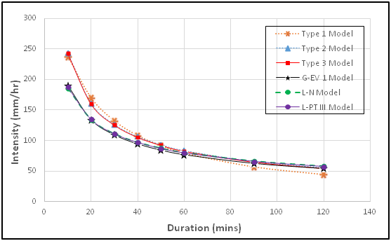
Figure 11 Distribution of nPDF and PDF IDF curves for Port Harcourt metropolis for 8 year return period.

Discussion

Developing PDF-IDF models: The purpose of this study was to derive IDF equations and develop IDF curves using both probability distribution function techniques and conventional empirical methods (nPDF models) to estimate the rainfall intensity for Port Harcourt metropolis that can serve as design tool for drainage sizing, storm management, economic and safe flood control measures. Five PDF models namely Gumbel EVT-1, Normal, Log-Normal, LPT-3 and PT-3 distributions were used for frequecncy analysis of rainfall data collected. The analysis applied Chow²³ formula for estimation of magnitude of rainfall intensity IDF curves for which rainfall estimates decreased with increase in duration and increased with increase in return period. The results obtained from the five PDFs methods showed small differences and had good consisitency as was reported by Elsebaie.¹³ Goodness of fit test carried out to ascertain the best option (model) among the PDFs showed that all the five distributions statistic were less than the critcal value at 5% significance level. Thus, the data fitted the distributions and can be considered reliant.

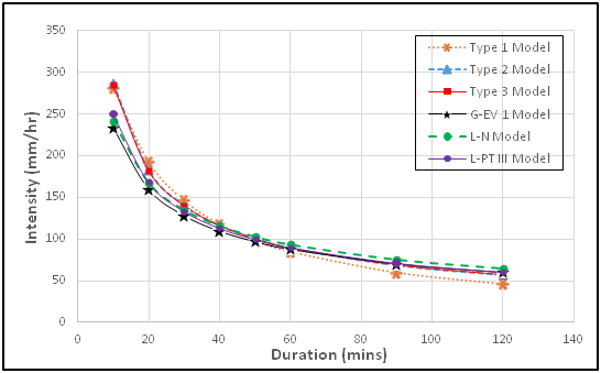
Figure 12 Distribution of nPDF and PDF IDF curves for Port Harcourt metropolis for 16 year return period.

The general rainfall PDF-IDF models and curves were further developed for the various PDFs. The general PDF-IDF models as in Figure 7 & Figure 8 predicted lower rainfall intensities for the five PDFs at lower return periods of 2, 5 and 10years, but predicted higher intensities at higher return periods of 25, 50 and 100 years. The predicted rainfall intensities obtained from the general PDF-IDF models relatively showed a good match with the computed rainfall intensity from the five PDFs. The predicted rainfall intensities plotted in arithmetic graph paper showed good closeness with some degree of parallelness for specified return periods. The PDF- IDF curve results show that by specifying rainfall return period or duration, intensity value can be obtained in agreement with publication in literature.^17,21 The goodness of fit, (R²) values obtained are all within the range of 0.961 to 0.975 indicating very high fit in each of the model. The mean squared error (MSE) also varied betweeen 92.71 and 256.84. Thus, the PDF-IDF model of choice should be the Normal distribution with MSE 92.71 and seconded by the Gumbel EVT-1 distribution with MSE of 109.39.

Comparative analysis of PDF and nPDF IDF models: The three PDF-IDF and nPDF-IDF models considered for comparative analysis were calibrated by non-linear regression analysis method for specified return periods of 2, 5, 8 and 16 years. The three nPDF–IDF model types selected were: Type 1 – Talbot simple quotient, Type 2 – power, and Type 3 – Sherman quotient-power models. While the PDF-IDF models selected were: Gumbel EVT-1, Log-Normal and LPT-3 models. The results of goodness of fit (R²) for nPDF–IDF models ranged between 0.864 and 0.996, while that of PDF-IDF models ranged between 0.967 and 0.997 which are clear indication that the variables have good correlationship. This relationship however are better exhibited in the PDF-IDF models which showed a stronger correlationship. The R² for the PDF-IDF at 2 and 5 year return periods gave: Gumbel EVT-1 0.992 - 0.997; Normal are 0.995 - 0.997; Log-Normal are 0.985-0.993; LPT-3 are 0.967-0.989; and PT-3 are 0.971-0.995, respectively. The mean squared error (MSE) results for the PDF-IDF showed consistency from lower values at 2 year return period to higher values at 16 year return period. The MSE for the PDF-IDF at 2 and 5 year return periods gave: Gumbel EVT-1 1.89-3.55; Normal are 1.66-4.33; Log-Normal are 2.41-5.97; LPT-3 are 4.63-9.15; and PT-3 are 5.69-5.85, respectively. In nPDF-IDF model, the Talbot-Type 1 equation gave MSE value varying from 8.77 at 2 year to 32.24 at 5 year return period. The Type 2 and 3 equations gave 18.53-45.53 at 2 and 5 years, each. The MSE and R² values of the PDF-IDF models showed that the models are better than those of nPDF-IDF models.

Furthermore, the comparative study of the IDF models sought to determine whether significant difference exist in the predicted intensity distribution between the three PDF and three nPDF-IDF models selected. The Kruskal Wallis non-parameter test was performed on two segments of the IDF model distribution, that is, for 10 – 40 minute and 50–120 minute durations. The results of the test shown in Table 6 indicated that the calculated K-values are less than the K critical at 0.05 level of significance. The P-values are also greater than alpha value of 0.05, therefore we accept the null hypothesis (i.e no significant difference exist). The result indicates that there are no significant differences found amongst the predicted intensities of the different IDF models (PDF & nPDF models).²⁸

Model derivation of PDF and nPDF-IDF types were accomplished using non-linear regression analysis with respect to model calibration and verification. Results of the derived IDF models are consistent with IDF theory of higher intensity occuring at lower duration and lower intensity occuring at higher duration. The intensity also increased with higher return period. The PDF-IDF models predicted rainfall intensities which showed a good match with the observed rainfall intensity from the five PDFs. The Normal distribtution model ranked as the best with respect to MSE=92.71 and R²=0.970 in the general PDF-IDF model category, while the Gumbel EVT-1 model was second best (MSE=109.39 and R²=0.975) and showed better result for each of the specified return periods (2, 5, 8 and 16 years). The nPDF-IDF models showed higher prediction at lower durations of 10 – 40 minutes, while the PDF–IDF models showed higher prediction at higher durations of 50 – 120 minutes. The nPDF-IDF models return period are limited by the number of years of data collection, while the PDF-IDF models predicted higher rainfall intensities for longer return period of 25, 50, and 100 years. There are no significant differences amongst the predicted intensities of the various IDF models compared (i.e PDF and nPDF models).

None.

The author declare that there is no conflicts of interest.

1. Akintola FO. The hydrological consequences of urbanization: a case study of Ibadan City. In: Sada & Oguntoyinbo, editors. Urbanization Process and Problems in Nigeria. University Press, Ibadan. 1978.
2. Omiunu FG. Ogunpa flood disaster: An environmental problem or a cultural fiction. Aman. 1981;100–120.
3. Meyer AF. The element of hydrology. John Wiley and Sons, Inc., New York, 2nd ed. 1928.
4. Sherman CW. Frequency and intensity of excessive rainfalls at Boston. Massachusetts Trans Am Soc Civil Engrs. 1931;95:951–960.
5. Bernard MM. Formulas for rainfall intensities of long durations. Transactions. ASCE. 1932;96:592–606.
6. Bilham EG. Classification of Heavy falls in short periods. British Rainfall 1935. 1963;262–280.
7. Holland DJ. Rainfall Intensity Frequency relationships in Britain. British Rainfall. 1967;43–51.
8. Hershfield DM. Estimating the Probable Maximum precipitation. Journal of the Hydraulic Division, Proceeding of the ASCE, HY5. 1961;87(5):99–116.
9. Bell FC. Generalized rainfall–duration–frequency relationship. Proceedings, ASCE, 95, HYI. 1969;311–327.
10. Chen CL. Rainfall Intensity Duration Frequency formulas. ASCE Journal of Hydraulic Engineering. 1983;109(12):1603–1621.
11. Bara M, Kohnova S, Gaal L, et al. Estimation of IDF curves of extreme rainfall by simple scaling in Slovakia. Contribution to Geophysics and Geodesy. 2009;39(3):187–206.
12. Alhassoun SA. Developing Empirical formulae to Estimate Rainfall Intensity in Riyadh Region. Journal of King Saud University – Engineering Sciences. 2011;23(2):81–88.
13. Elsebaie IH. Developing rainfall intensity–duration frequency relationship for two regions in Saudi Arabia. Journal of King Saud University Engineering Sciences. 2012;24(2):131–140.
14. Oyebande L. Deriving Rainfall Intensity–Duration–Frequency Relationships and Estimates for regions with inadequate Data. Hydrological Sciences Journal. 1982;27(3):353–367.
15. Nwaogazie IL, Duru EO. Developing Rainfall Intensity–Duration– Frequency models for Port Harcourt City. Nig Society of Engineers Technical Transaction. 2002;37(2):19–32.
16. Nwaogazie IL, Uba LO. Urban Drainage Failures and Incidence of Flooding in Southern Nigeria. NSE Technical Transactions. 2001;36(3):43–53.
17. Nwaogazie IL, Ologhadien I. Rainfall intensity – duration – frequency models for selected cities in Southern Nigeria. Standard Scientific Research and Essays. 2014;2(10):509–515.
18. Okonkwo GI, Mbajiorgu CC. Rainfall intensity – duration –frequency for South Eastern Nigeria. Agriculture Engineering International CIGRE Journal. 2010;12(1):22–30.
19. Akpan SU, Okoro BC. Developing rainfall intensity duration Frequency models for Calabar city, south–south, Nigeria. American Journal of Engineering Research (AJER). 2013;2(6):19–24.
20. Akpen GD, Aho MI, Ojo OG. Rainfall Intensity–Duration–Frequency models for Makurdi metropolis, Nigeria. International Journal of Scientific and Engineering Research. 2016;7(5):838–849.
21. Nwaogazie IL, Okonkwo SC. Rainfall–Intensity–Duration–Frequency Modeling and Comparative Analysis of Developed models for Abakiliki, Ebonyi State, Nigeria. International Journal of Trend in Research and Development. 2017;4(2):2394–9333.
22. Gobo AE. Rainfall Data Analysis as an Aid for Maximum Drainage and Flood Control Works in Port Harcourt. The Journal of Discovery and Innovation, Nairobi. 1990;2(4):25–31.
23. Chow VT. A General Formula for Hydrologic Frequency Analysis. Trans Amer Geophys Union. 1951;32:231–237.
24. Chow VT, Maidment DR, Mays LW. Applied Hydrology. 1st ed. McGraw –Hill, New York. 1988.
25. Raghunath HM. Hydrology: Principles, Analysis and Design. 2nd ed, New Age International Publishers. Delhi. 2006.
26. Zakwan Mohammad. Application of Optimization Techniques to Estimate IDF Parameters. Water and Energy Research Digest (Water Resources Section). Research Gate Journal. 2016;1–3.
27. Spielgel MR. Schaum’s Outline Series (1972): Theory and problem of statistics. SI (Metric) edition; Mchraw–Hill Book Company. 1972.
28. Chen W, Fand Richard JY. The Civil Engineering Handbook. 2nd ed. CRC Press LLLC, New York. 2003.