Landslide is one of the most destructive natural hazards that can impose economical and life loss. Fortunately, through numerical and spatial analysis we can lessen the damages caused by landslides. In this study which goes through landslide susceptibility mapping, a combination of AHP and Fuzzy approaches is applied. AHP is used in order to prioritize the effective criteria and Fuzzy method is used in two steps, factor map fuzzification, and factor maps are calculated and overlaid after fuzzification. In order to achieve the best output susceptibility map, 6 scenarios has been proposed in fuzzy overlay step for a study area in Iran as a case study and the best scenario has been chosen according to the comparison of every output with observed landslides layer. The susceptibility map that has the greatest overlap area was the result of using fuzzy Or in overlap step which is considered as a suitable way in hazard risk zonnation. Analysis of the final landslide susceptibility map shows that scenario 6 which is proven to be the most suitable outcome, has the least AUC= 0.3 and matches with observed landslides much better than other scenarios, and through physiographical analysis, we found that most landslides have occurred and are probable in are used as good ranges, are in middle slope angle, and have northern slope aspects.

Keywords: Landslide Modelling, Site selection, GIS, AHP, Fuzzy, Iran

Landslide which is defined as the movement of a mass of rock, debris or earth down a slope,¹ is known as one of the most destructive natural hazards all over the world² but fortunately, it can be prevented through different available methods including prediction and wise constructions. Damages caused by landslides can be ranging from top soil loss to human death, they also can change the figure of the landscape such as causing landslide dams that occur when a huge landslide blocks a river flow and causes a lake,³ this type of dam frequently occurs in tectonically active mountains which cause sudden landslides.⁴ In case of losing top soil, the problem doubles when the removed soil is carried into the reservoir of a dam which can occupy a big proportion of its capacity. Landslides can have an impact on forests in a way that tree biomass would recover between 80-200 years⁵ that means the damaged area will be bare for a long time. Different landslide classifications have been released in case of landslides, however, the most reliable and famous classification is done by Warnes⁶ in which landslides are primarily classified by the type of movement. The cohesion and friction forces of rocks and soils prevent the slopes from moving down due to gravity, however, sometimes because of a variety of causes, the adjustment of the equilibrium fails and it results in a landslide.⁷ Landslides might be either natural or human induced⁸ also depending on the geographical and climatic conditions, both kinds of triggers can cooperate and cause a landslide. There are some major factors such as unfavorable geology, rise in underground water and heavy rainfall during few days before the movement,⁹ there are also a vast number of factors which with a relatively difference in importance, can cause a landslide these factors can be listed as constructions, slope angle, slope aspect, curvature of the slope, distance to fault, climate condition^10,11 land cover¹² etc. Depending on the region, the importance of each factor might be lower or higher than others. Many studies have been applied to know the landslides better also to understand how to minimize the direct and indirect costs and prevent them. Landslide susceptibility maps are helpful tools for decision makers and future constructors for spatial plannings,¹³ therefore many different approaches have been applied to make the most optimum prediction of landslide disasters, some examples of these approaches are Index of Entropy (IOE)¹⁴ Weigh of Evidence¹⁵ Statistical Index method,¹⁶ Logistic Regression^4,16,17 Analytic Hierarchy Process technique^16,18,19 Fuzzy Logic.^20–23 Barrile et al.²⁴ used GIS-based fuzzy logic in order for road network planning.²⁴ Feizizadeh et al.²³ applied fuzzy and AHP approaches for landslide susceptibility mapping and the output was considered as satisfactory due to 53% overlap with observed landslide layer.²⁵ Bui et al. used the GIS-based fuzzy neural network for landslide susceptibility mapping and through testing multiple membership functions figured out that Gaussian membership function was the most suitable function Kayastha et al.²⁶ applied AHP for landslide susceptibility mapping and according to the reliable outcome, they considered AHP as a reasonable approach Althuwaynee et al.²⁷ compared AHP Logistic regression, and Bayesian methods in landslide susceptibility mapping, and found AHP as the most reliable method for criteria rating. Wang et al.²⁸ applied three methods (multi-criteria statistical analysis, logistic regression, and multivariate adaptive regression spline models) and the results showed that the last method which had 77% overlap with observed landslides map, had the most productivity among other methods.²⁸ Poiraud used 5 methods (Indicator, weight-of-evidence, logistic regression, decision tree, one condition unit) to obtain landslide susceptibility map and since all outcomes were reliable, he used the combination of all results as the final outcome that highly matched with observed landslide layer.²⁹ Ciurleo et al.³⁰ used statistical methods for landslide susceptibility mapping in small and big scales and found out that although all the methods show reliable results, a bigger scale mapping is more reasonable because more criteria can be considered.³⁰ In order to obtain landslide susceptibility map, Erener et al.³¹ tested logistic regression, GIS-based multi criteria analysis, and Association Rule Mining and through the validations realized that logistic regression and ARM method had better outcome.³¹ Keh-Jian Shou considered climate as a dynamic criteria and used logistic regression in order to obtain a landslide susceptibility map for each rainfall scenario.³² Pradhan et al.³³ applied spatial multi-criteria evaluation model and deterministic model for landslide susceptibility mapping and after combining the results of two methods achieved a reliable outcome of 79.59% matching.³³ Shahabi et al. applied landslide susceptibility mapping through AHP, logistic regression, and Frequency Ratio methods and realized that logistic regression and Frequency Ratio have more reliable results.³⁴ Hong et al.³⁵ applied GIS-based Frequency Ratio method for landslide susceptibility mapping and achieved a reasonable accuracy of 80.5% which showed the reliability of the results.³⁶ In this paper, according to the optimum results recognized in literature and high accuracy of combined methods in landslide susceptibility mapping, GIS based Fuzzy Logic is used in calculations and overlays and AHP approach is applied in order to allocate weights to the factors.^37,38

The following steps were applied in order to reach the final susceptibility map:

1. Collecting and rectifying the effective factor maps
2. Applying AHP approach in order to estimate the weight of each factor
3. Fuzzification and application of the weights to each layer using GIS
4. Overlaying all the spatial data and generating the final landslide susceptibility map
5. Validation through comparing the high susceptibility zones with the landslide inventory map

Criteria defining and localizing

In every study, the basic and first step is to build a dataset for criteria which is specifically designed for the study area. In this study, based on the surveys and researches, nine criteria were selected (precipitation,³⁹ slope,^39–43 aspect,^39–43 lithology,^{21,39,40,43,44} landuse,^40–46 distance to road,^39–42 distance to river,^39,41 distance to faults,^39,43 and curvature.^39–42 In order to produce and analyze the data layers, ArcGIS was used and all factors were prepared as a raster dataset. Basic data were collected from organizations in charge of natural resources studies and management and were adapted and matched together to obtain the best possible result.

Analytic hierarchy process

Analytic Hierarchy Process (AHP) is a Multi Criteria Decision Making (MCDM) method that was originally developed by Prof Thomas L Saaty⁴⁵ AHP is one of the most suitable approaches for decision making because in natural phenomena all the factors depend on the other factors and when it comes to natural analysis, it is not logical to consider them as independent factors. Based on the pairwise comparison in AHP approach we can be positive about the weighs that are allocated to each factor. In order to apply AHP these steps were followed:

    Preparing a pairwise comparison questionnaire to ask experts' opinions in an scale between 1 to 19.

    Analyzing the results in a comparison matrix for all criteria and sub-criteria

    Extracting priority weights for each factor

Fuzzy method

Fuzzy set theory is a very helpful approach to model complex systems that are not logical to be defined by crisp numbers. A fuzzy set theory which was introduced by Zadeh⁴⁶ makes researchers capable of analyzing the smooth and vague changes in a set rather than crisp boundaries for changes especially in natural conditions because many spatial phenomena such as factors that affect landslide don't have value boundaries. In fuzzy set theory, each object or pixel can have a membership value between 0 and 1 which reflects a degree of membership.⁴⁶ In this theory each object is affected by its left and right side according to two kinds of membership functions:

1. Linear membership function and
2. Bsinusoidal membership function. In this study the sinusoidal function has been applied (here the precipitation fuzzy set is shown as an example)

${\mu }_{precipitation}\left(x\right)=\{\begin{array}{l}0x\le {100}_{mm}\\ \frac{1}{2}\left(1-\cos \left(\pi \frac{x-100}{250}\right)\right)100<x\le 450\\ \frac{1}{2}\left(1-\cos \left(\pi \frac{x-450}{350}\right)\right)450<x\le 800\\ \frac{1}{2}\left(1-\cos \left(\pi \frac{x-800}{350}\right)\right)800<x\le 1150\\ 11150<x\end{array}$

Application of fuzzy and AHP

In order to apply the methods on spatial maps that result in achieving the landslide susceptibility map, ArcGIS has been used by this order:

      Fuzzification

      Applying weights for each main factor as well as each class

      Overlaying layers

       Validating of the final result through comparison with previously observed landslide (inventory)

The study area is the lands upper side of Taleghan dam basin which is in the northwest of Alborz province. The catchment is a mountainous and elevated area in central Alborz mountain range with north latitudes of 36˚ 5' 40" to 36˚ 21' 5" and east longitudes of 50˚ 36' 40" to 51˚ 11' 16" as shown in Figure 1. The study area is about 960 Km² with a perimeter of 161 Km, a length of 51 Km average elevation of 3045 m, and the lowest point, located at the Taleghan dam, 1688m.³⁶ The climate of Taleghan County is mountainous cold with almost high amount of precipitation (Figure 2). Figure 3 shows the climate map of Taleghan. According to the location of the area which is between northern Alborz with highly humid and cold and southern Alborz with almost dry climate. Taleghan area has always been suitable for nomads whose life is based on keeping livestock, therefore large parts of the area are used as range. In recent years and since the construction of the dam, many residences have tended to have orchards, as shown in Figure 4 that shows land use map of Taleghan. Regarding the geological structure, the area is made of a vast combination of the hard and easily destroyed type of land. For example, the southern hillside is mostly silt and gypsum which are highly landslide prone and northern side with the volcanic rocks is more slide resistant.³⁷ Figure 5 shows geology map of Taleghan. Regarding the tectonic situation, Taleghan hosts a major active fault called Taleghan Fault which has historically caused many earthquakes in the area,³⁸ there are also many semi active and inactive faults that cover all over the area. Based on the previous landslide events and observations it can be said that many of them have been tectonic caused, therefore faults have a major role in predicting future landslides.

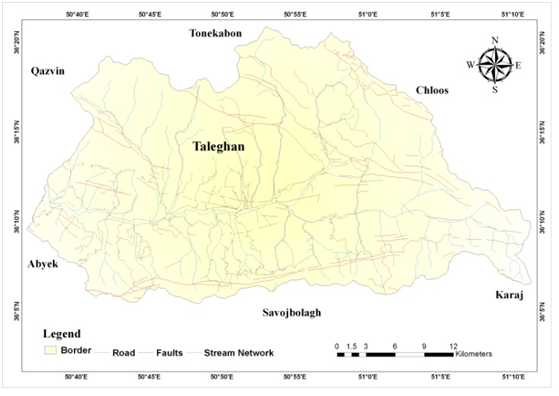
Figure 1 General Map of Taleghan (Study area).

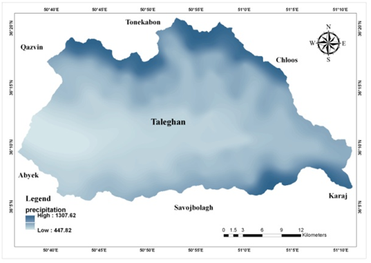
Figure 2 Precipitation map of Taleghan.

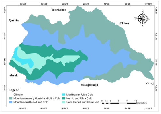
Figure 3 Climate map of Taleghan.

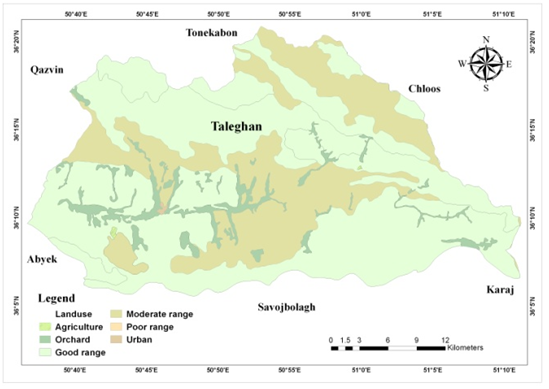
Figure 4 Landuse Map of Taleghan.

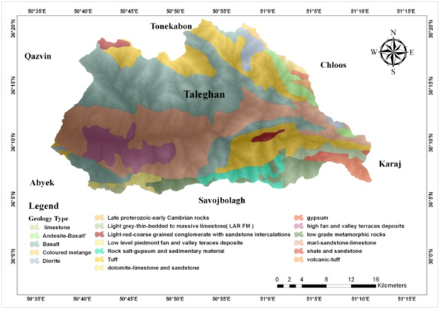
Figure 5 Geology Map of Taleghan.

The research aims to model the susceptibility of landslide hazard in a highly landslide prone area through integrating two approaches which are historically helpful in analyzing natural phenomena. we applied AHP because of its proved advantages in decision making that can be obtained through pairwise comparison. Also, Fuzzy set theory which is appropriate for spatial and natural phenomena because of omitting the crisp boundaries is used. Results of AHP analysis are given in Tables 1–3.

Conceptual model

The process of the study is shown through the conceptual model as follow (Figure 6):

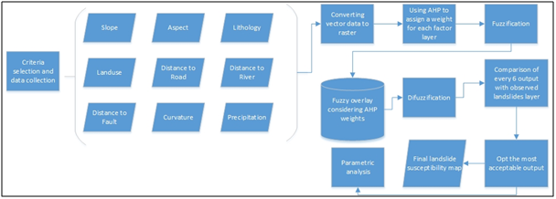
Figure 6 The flow diagram of the study.

In the fuzzification step, using the fuzzy membership function rules, a membership function has been applied for each factor as follow:

${\mu }_{precipitation}\left(x\right)=\{\begin{array}{l}0x\le {100}_{mm}\\ \frac{1}{2}\left(1-\cos \left(\pi \frac{x-100}{250}\right)\right)100<x\le 1150\\ 11150<x\end{array}$

${\mu }_{slopeangle}\left(x\right)=\{\begin{array}{l}0x\le 2\\ \frac{1}{2}\left(1-\cos \left(\pi \frac{x-2}{73}\right)\right)\text{ 65}<x\le 75\\ 1\text{ 7}5<x\end{array}$

${\mu }_{slopeangle}\left(x\right)=\{\begin{array}{l}01\\ \frac{1}{2} \left(1-\cos \left( \pi \frac{180-x}{180}\right)\right) 0<x\le 180\\ \frac{1}{2} \left(1-\cos \left( \pi \frac{x-180}{180}\right)\right) 180<x\\ 1\text{ 80 }0\end{array}$

In order to fuzzify the slope aspect map, we assume that northern slopes receive less light and are damper than southern slopes, therefore from 0 to 180-degree azimuth was considered as increasing membership and 180 to 360, in contrast, was considered as decreasing membership.

${\mu }_o{}_{distance to river}\left(x\right)=\{\begin{array}{l}01000<x\\ \frac{1}{2} \left(1-\cos \left( \pi \frac{x-50}{200}\right)\right) 50<x \le 1000\\ 1\text{ 80 }0\end{array}$

${\mu }_{distance to road}\left(x\right)=\{\begin{array}{l}01000<x\\ \frac{1}{2} \left(1-\cos \left( \pi \frac{x-100}{900}\right)\right) 100<x \le 1000\\ 1\text{ x<10}0\end{array}$

${\mu }_{distance to fault}\left(x\right)=\{\begin{array}{l}0\text{ x>}1000\\ \frac{1}{2} \left(1-\cos \left( \pi \frac{x-100}{900}\right)\right) 1000<x \le 100\\ 1\text{ x<10}0\end{array}$

${\mu }_{curvature}\left(x\right)=\{\begin{array}{l}\frac{1}{2} \left(1-\cos \left( \pi *-\left(\frac{x- 3.12}{ 3.12}\right)\right)\right) x\le 0\\ \frac{1}{2} \left(1-\cos \left( \pi \frac{ 3.09-x}{3.09}\right)\right) 0<x\end{array}$

Fizzification results are given in Figures 7‒13. Through fuzzy overlaying, 6 final results have been obtained using 6 different overlaying scenarios in order to choose the best susceptibility map which has the highest overlap with observed landslide map (Figure 14). In this step, all the factor maps were overlaid using an average value of gamma. The output of scenario 1 is given in Figure 15. In scenario 2 we assumed to set a maximum value of each factor group at the first step and set a minimum value in the second step that combines the results of the previous combination, accordingly there could be a balance of values (Figure 16). Output layer of this scenario in given in Figure 17. In scenario 3, the values have a tendency to be chosen as a minimum (Figure 18), and it is applied through using gamma functions. The output of scenario3 is given in Figure 19. In scenario 4, in the case of physiographic and human induced factors, because of the high influence of land use and distance to fault, fuzzy and operator was used to keep the highest values (Figure 20). The output of this scenario in given in Figure 21. Scenario 5 was applied in order to take distance to river and distance to fault as geological factors because the formation of the slopes which can be near or distant from natural triggers is based on their geology (Figure 22). In the other hand precipitation as a climatic factor which provides abrupt trigger was considered as an independent factor. Output layer of this scenario is given in Figure 23. In the last scenario, a minimum of all the values was aimed and distance to the road was considered as a location based factor (Figure 24). Output layer of this scenario is given in Figure 25. Each output layer of all the scenarios were compared with the observed landslides layer which is shown in Figure 26 in order to opt the best match between highly susceptible areas and the areas that have actually experienced landslide, and the results are provided in Tables 4–9.

Figure 7 Fuzzy slope map of Taleghan.

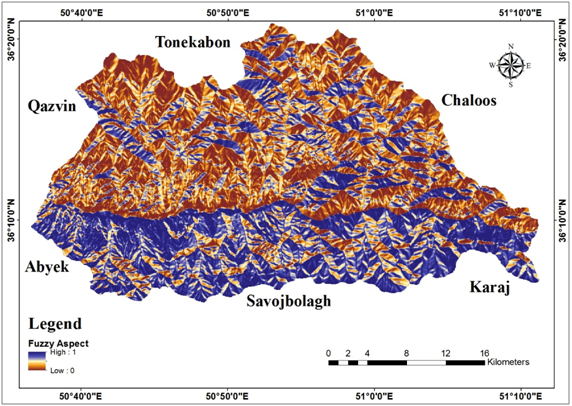
Figure 8 Fuzzy aspect map of Taleghan.

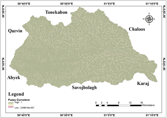
Figure 9 Fuzzy curvature map of Taleghan.

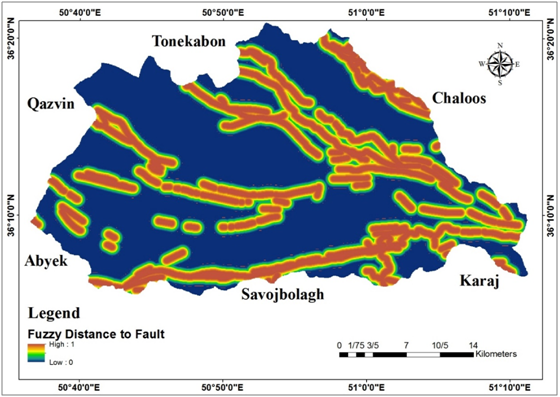
Figure 10 Fuzzy distance to road map of Taleghan.

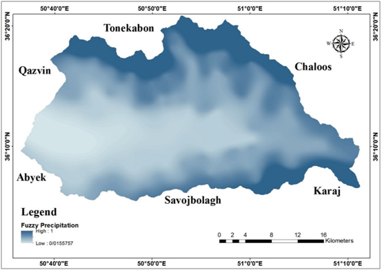
Figure 11 Fuzzy precipitation map of Taleghan.

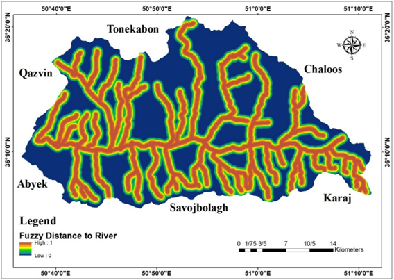
Figure 12 Fuzzy distance to river map of Taleghan.

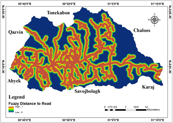
Figure 13 Fuzzy distance to road map of Taleghan.

Figure 14 scenarios 1 Layers and overlaying.

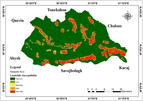
Figure 15 Landslide susceptibility according to scenario 1.

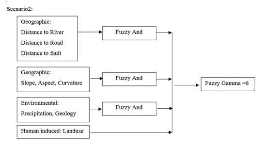
Figure 16 Scenarios 2 Layers and overlaying.

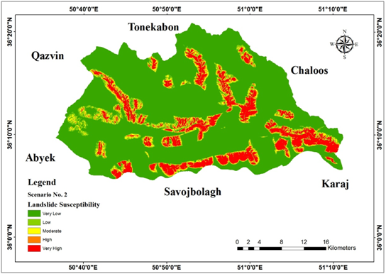
Figure 17 Llandslide susceptibility according to scenario 2.

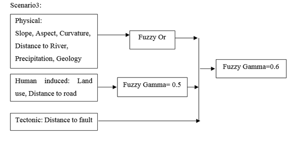
Figure 18 Scenarios 3 Layers and overlaying.

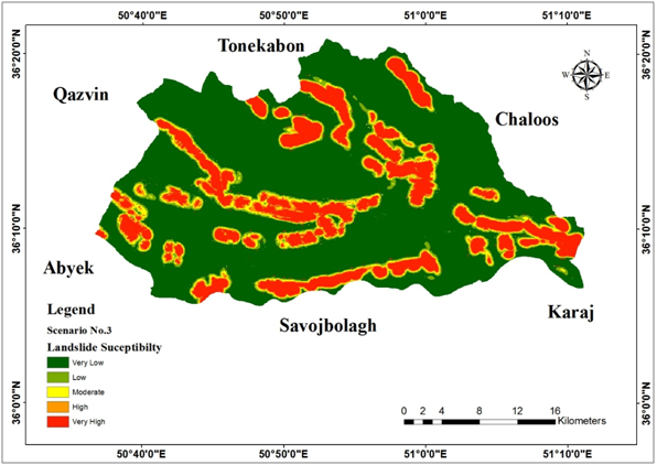
Figure 19 Landslide susceptibility according to scenario 3.

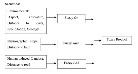
Figure 20 Scenarios 4 Layers and overlaying.

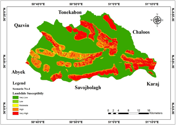
Figure 21 Landslide susceptibility according to scenario 4.

Figure 22 Scenarios 5 Layers and overlaying.

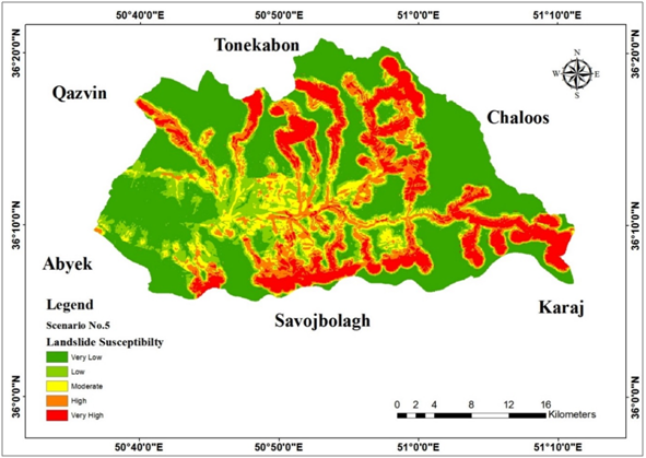
Figure 23 Landslide susceptibility according to scenario 5.

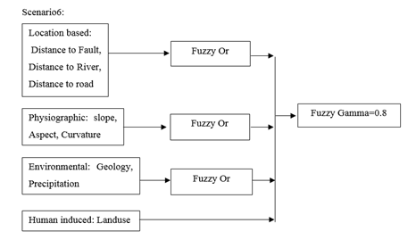
Figure 24 Scenarios 6 Layers and overlaying.

Figure 25 Landslide susceptibility according to scenario 6.

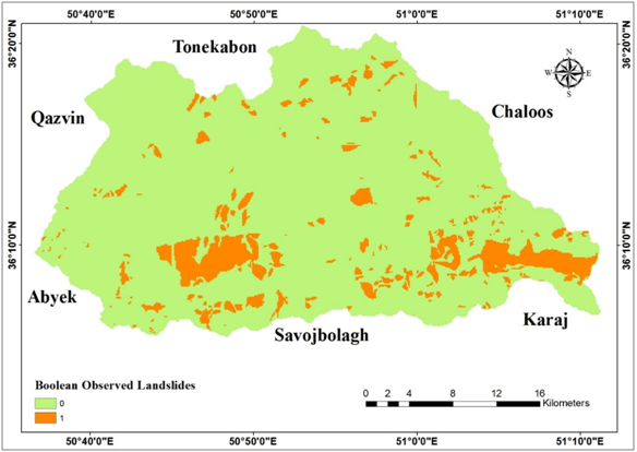
Figure 26 Observed landslides in study area.

In order to weigh up the assumed scenarios and opt the best suited output, the accumulative ratio of observed landslide area in each susceptibility level was calculated and plotted as it is shown in Figure 27. The plot illustrates the accumulation of actual landslide occurrence in each susceptibility level of every assumed scenario. A general look at the plot shows that there is an abrupt increase in high susceptibility which resembles the fact that areas that experienced landslide in the past are highly potential to experience it in the future again.

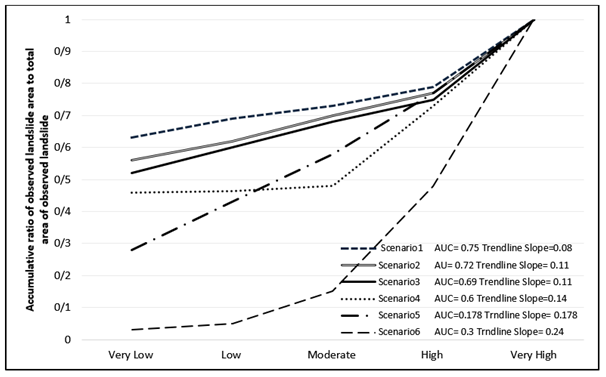
Figure 27 Observed landslides in study area.

A more mathematical look at the plot reveals that area under the curve (AUC) has decreased in scenarios from 1 to 6, which shows a gradual rise in observed landslides in each susceptibility level. Trend line's steepness was also considered as a comparison factor because it is completely reasonable that the least susceptible area must have experienced the least landslide events, and having this in mind, it is clear that scenario 6 proves to be the best fit model among assumed scenarios. Through an overview of the fuzzy operators we used in each scenario, it can be found out that as it is believed, using fuzzy Or to overlay fuzzy factor maps is reliable. Parametric analysis shows that in the case of landuse which is shown in Figure 28 there is a relatively likelihood between output susceptibility map and observed landslides. As it is clear in the plot, the good range includes the most landslide history and the highest possibility of landslide occurrence, it can be caused by many approximately active faults which lie in this part of the study area. Through a look at slope angle comparison between simulated landslides and observed landslide, it can be clearly noticed that as it is shown in Figure 29 there is no significant difference between them and it can be concluded that mostly landslides occur in middle slope angles. Analysis of geographical aspect in both simulated landslide and observed landslide which is given in Figure 30 shows that the assumption that northern slopes are more susceptible to landslide occurrence is highly true because in both layers they include more landslide areas than other aspects.

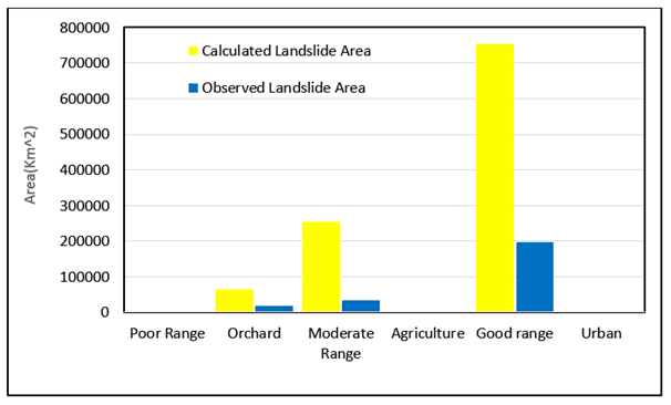
Figure 28 Landslides in each landuse type.

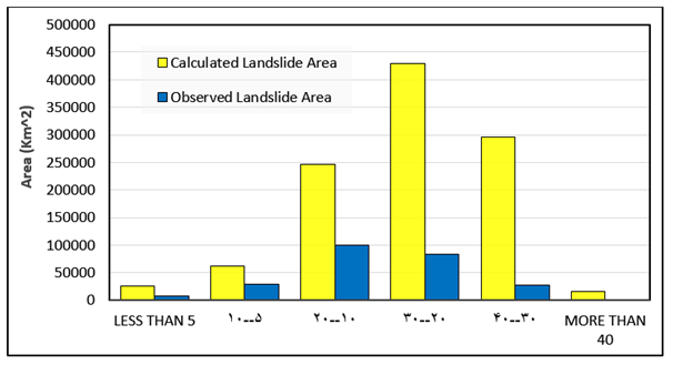
Figure 29 Landslides in different slope percent.

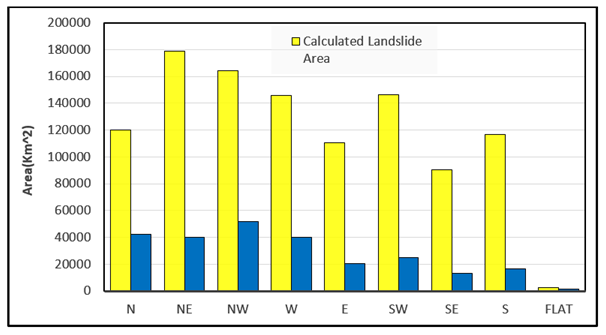
Figure 30 Landslides in each slope aspect.

In this study, the susceptibility of landslide in Taleghan watershed was studied using AHP and FUZZY methods in GIS environment through considering factors such as geology, landuse, slope, aspect, precipitation, distance to road, distance to fault, distance to river, and curvature. Factors were chosen according to the literature and previous studies. AHP method was applied to assign the weight of each factor in causing landslide and through fuzzy method factor maps were fuzzified where possible. In the case of landuse and geology that fuzzification was not possible, AHP results were used because changes are not gradual. In order to overlay the data layers, 6 scenarios were assumed, that scenario 6 was proved the best suitability according to the AUC=0.3 and trend line slope =0.24. Through comparison between susceptibility map obtained from the study and observed landslides, it can be clearly concluded that output of the study is reliable and it can be used as a basis for future studies and safety plannings. Analysis of physiographical factors shows that in both observed landslide map and susceptibility map, mostly landslides occur in northern aspects, middle slope angles, and good rangs. Physiographical analysis of the results emphasize on the concept that in natural events there is not just one major cause for a hazard and depending on other conditions there can be different intensity in factors' roles. Nature is dynamic and changes permanently, therefore in order to be able to reduce the losses in natural hazards such as landslides we have to use previous studies as a basis for new approaches and methods. We hope that this study will be continued with future studies.

None.

None.

1. Cruden DM. A simple definition of a landslide. Bulletin of the International Association of Engineering Geology. 1991;43:27–29.
2. Alimohammadlou Y, Najafi A, Yalcin A. Landslide process and impacts: A proposed classification method. Catena. 2013;104:219–232.
3. Highland LM, Bobrowsky P. The landslide handbook—A guide to understanding landslides. Reston, Virginia, US Geological Survey Circular; 2008. p. 1–147.
4. Xuanmei F, Cees JVW, Qiang Xu, et al. Analysis of landslide dams induced by the 2008 Wenchuan earthquake. Journal of Asian Earth Sciences. 2012;57:25–37.
5. Dislicha C, Hutha A. Modelling the impact of shallow landslides on forest structure in tropical montane forests. Ecological Modelling. 2012;239:40–53.
6. Hungr O, Leroueil S, Picarelli L. The Varnes classification of landslide types, an update. Landslides. 2014;11(2):167–194.
7. De Blasio FV. Introduction to the Physics of Landslides. Netherlands: Lecture Notes on the Dynamics of Mass Wasting; 2011. p. 408.
8. Hancox GT. The 1979 Abbotsford Landslide, Dunedin, New Zealand: a retrospective look at its nature and causes. Landslides. 2008;5(2):177–188.
9. Tim Davies, Shroder JF. Landslide Hazards, Risks, and Disasters. In: Samuel T, Mc Coll, editors. Landslide Causes and Triggers. Elsevier. 2015:17–42.
10. Flageollet J, Maquaire O, Martin B, et al. Landslides and climatic conditions in the Barcelonnette and Vars basins (Southern French Alps, France). Geomorphology. 1999;30(1–2):65–78.
11. Noorollahi Y. Application of GIS and remote sensing in exploration and environmental management of Namafjall geothermal area, N–Iceland. MSc thesis, University of Iceland, Reykjavik: UNU–GTP report 1; 2005. p. 1–124.
12. Rickli C, Graf F. Effects of forests on shallow landslides – case studies in Switzerland. For Snow Landsc Res. 2009;82(1):33–44.
13. Andersson SY, Bergman R, Johansson M, et al. Landslide risk management—A brief overview and example from Sweden of current situation and climate change. International Journal of Disaster Risk Reduction. 2003;3:44–61.
14. Pourghasemi H, Mohammady M, Pradhan B. Landslide susceptibility mapping using index of entropy and conditional probability models in GIS: Safarood Basin, Iran. CATENA. 2012;97:71–84.
15. Piacentini D, Troiani F, Soldati M, et al. Statistical analysis for assessing shallow–landslide susceptibility in South Tyrol (south–eastern Alps, Italy). Geomorphology. 2012;151:196–206.
16. Zhang G, Cai Y, Zheng Z, et al. Integration of the Statistical Index Method and the Analytic Hierarchy Process technique for the assessment of landslide susceptibility in Huizhou, China. Catena. 2016;142:233–244.
17. Kavzoglu T, Kutlug SE, Colkesen I. Selecting optimal conditioning factors in shallow translational landslide susceptibility mapping using genetic algorithm. Engineering Geology. 2015;192:101–112.
18. Wang L, Sawada K, Moriguchi S. Landslide susceptibility analysis with logistic regression model based on FCM sampling strategy. Computers &Geosciences. 2013;57:81–92.
19. Kiavarz MM, Noorollahi Y, Samadzadegan F, et al. Spatial data analysis for exploration of regional scale geothermal resources. Journal of Volcanology and Geothermal Research. 2013;266:69–83.
20. Banerjee S, Rondoni L, Mitra M. Applications of Chaos and Nonlinear Dynamics in Science and Engineering: Vol 2. Understanding Complex Systems. Springer–Verlag Berlin Heidelberg; 2012. p. 1–270.
21. Kayastha P, MAN Bijukchhen S, Raj DM, et al. GIS Based Landslide Susceptibility Mapping using a Fuzzy Logic Approach: A Case Study from Ghurmi–Dhad Khola Area, Eastern Nepal. Journal Geological Society of India. 2013;82(3):249–261.
22. Zhu A, Wang R, Qiao J, et al. An expert knowledge–based approach to landslide susceptibility mapping using GIS and fuzzy logic. Geomorphology. 2014;214:128–138.
23. Feizizadeh B, Shadman RM, Jankowski P, et al. A GIS–based extended fuzzy multi–criteria evaluation for landslide susceptibility mapping. Computers &Geosciences. 2014;73:208–221.
24. Barrile V, Cirianni F, Leonardi G, et al. Afuzzy–based methodology for Landslide Susceptibility Mapping. Procedia – Social and Behavioral Sciences. 2016;223:896–902.
25. Tien BD, Pradhan B, Lofman O, et al. Landslide susceptibility mapping at Hoa Binh province (Vietnam) using an adaptive neuro–fuzzy inference system and GIS. Computers & Geosciences. 2012;45:199–211.
26. Kayastha P, Dhital MR, De Smedt F. Application of the analytical hierarchy process (AHP) for landslide susceptibility mapping: A case study from the Tinau watershed, west Nepal. Computers & Geosciences. 2013;52:398–408.
27. Althuwaynee FO, Pradhan B, Park H, et al. A novel ensemble bivariate statistical evidential belief function with knowledge–based analytical hierarchy process and multivariate statistical logistic regression for landslide susceptibility mapping. Catena. 2014;114:21–36.
28. Wang L, Guo M, Sawada K, et al. Landslide susceptibility mapping in Mizunami City, Japan: A comparison between logistic regression, bivariate statistical analysis, and multivariate adaptive regression spline models. Catena. 2015;135:271–282.
29. Poiraud A. Landslide susceptibility–certainty mapping by a multi–method approach: A case study in the Tertiary basin of Puy–en–Velay (Massif central, France). Geomorphology. 2014;216:208–224.
30. Ciurleo M, Calvello M, Cascini L. Susceptibility zoning of shallow landslides in fine grained soils by statistical methods. Catena. 2014;139:250–264.
31. Erener A, Mutlu A, Sebnem DH. A comparative study for landslide susceptibility mapping using GIS–based multi–criteria decision analysis (MCDA), logistic regression (LR) and association rule mining (ARM). Engineering Geology. 2015;203:45–55.
32. Shou K, Yang C. Predictive analysis of landslide susceptibility under climate change conditions — A study on the Chingshui River Watershed of Taiwan. Engineering Geology. 2015;192:46–62.
33. Pradhan AMS, Kim YT. Evaluation of a combined spatial multi–criteria evaluation model and deterministic model for landslide susceptibility mapping. Catena. 2016;140:125–139.
34. Himan S, Saeed K, Baharin BA, et al. Landslide susceptibilitymapping at central Zab basin, Iran: A comparison between analytical hierarchy process, frequency ratio, and logistic regression models. Catena. 2014;115:55–70.
35. Hong H, Xu C, Tien BD. Landslide Susceptibility Assessment at the Xiushui Area (China) Using Frequency Ratio Model. Procedia Earth and Planetary Science. 2015;15:513–517.
36. Schleiss AJ, Boes RM. Dams and Reservoirs under Changing Challenges. Switzerland: CRC Press; 2011. p. 1–906.
37. Ghorbani M, Ahmadi A, Tiepolo M, et al. Clinopyroxene chemistry in Tertiary alkaline volcanic rocks from Taleghan, central Alborz, Iran: Implications for two parental melts. Chemie der Erde. 2013;73:565–568.
38. Nazari H, Ritz JF, Salamati R, et al. Morphological and palaeoseismological analysis along the Taleghan fault (Central Alborz, Iran). Geophysical Journal. 2009;178(2):1028–1041.
39. Mathie E, McInnes R, Fairbank H, et al. Landslides and Climate Change: Challenges and Solutions. In: Malet JP, Remaître A, et al. editors. UK:Assessing the influence of climate change on the activity of landslides in the Ubaye Valley; 2007. p. 21–24.
40. Mondal S, Maiti SR. Integrating the Analytical Hierarchy Process (AHP) and the Frequency Ratio (FR) Model in Landslide Susceptibility Mapping of Shiv–khola Watershed, Darjeeling Himalaya. Disaster Risk Sci. 2013;4:200–212.
41. Meten M, Prakash BN, Yatabe R. Effect of Landslide Factor Combinations on the Prediction Accuracy of Landslide Susceptibility Maps in the Blue Nile Gorge of Central Ethiopia. Geoenvironmental Disasters. 2015;2:9.
42. Romer C, Ferentinou M. Shallow landslide susceptibility assessment in a semiarid environment — A Quaternary catchment of KwaZulu–Natal, South Africa. Engineering Geology. 2016;201:29–44.
43. Pathak D. Knowledge based landslide susceptibility mapping in the Himalayas. Geoenvironmental Disasters. 2016;3:8.
44. Wang M, Liu M, Yang S, et al. Incorporating Triggering and Environmental Factors in the Analysis of Earthquake–Induced Landslide Hazards. Disaster Risk Sci. 2014;5(2):125–135.
45. Saaty T. Decision making with the analytic hierarchy process. Int J Services Sciences. 2008;1(1):83–98.
46. Zadeh L. Fuzzy Sets. Information Control. 1965;8(3):338–353.