Electromagnetic wave data are simulated in representation of waves registered by a Ground Penetrating Radar (GPR), post-stacked and migrated, by convolving the synthetic electric permittivity of a model of parallel layers of soil and a ricker wavelet. Data well information of synthetic electrical permittivity is perturbed close to the original synthetic data on electric permittivity properties associated to a model conformed with parallel layers. We define a priori probability density function on the space of models, then use Bayes theorem to combine this probability with the data misfit function into a final a posteriori probability density reflecting both data fit and model reasonableness, we incorporate the covariance matrix of the well data and synthetic data. The posteriori probability is optimized via a nonlinear scaled conjugate gradient. The input data of the scaled conjugate gradient algorithm are the well permittivity electric data, the Ground Penetrating Radar source wavelet (Ricker) and the synthetic electromagnetic wave data that represents the waves recorded by a GPR post-stacked and migrated are contaminated with 5% noise and without noise. The SCG algorithm is initialized to an average constant value of the well data.

The results obtained from the inversion are very close to the initial real synthetic values of the electric permittivity model of parallel layers of the soil, that we wanted to recover, via this proposed inversion technique.

Keywords: simulation, electromagnetics wave propagation, electric permittivity

Geophysical data inversion deals with the problem of a quantitative inference on Earth model parameters from data observation. One sound approach to this problem is what is called the Bayesian inference method, where a priori information on the Earth parameters is known in terms of its probability distribution function sand new data is sought to improve the knowledge of Earth Model parameters in terms of a better constrained a posteriori probability distribution functions of those very same parameters. In this work we apply the Bayesian approach to electric permittivity data where we believe that a priori information can reasonably be derived from in situ petrophysical/field measurements. Therefore, due to observations are subject to uncertainty, these inferences are inherently probabilistic. Also, due to the epistemic error associated to uncertainties in the model parameters, this call for a framework which includes both a model for the random noise associated to the capturing of the data and the one associated to the lack of certain knowledge on the fabrics on the Earth media. Therefore, our task is to find an improved Earth model that fits new collected data, but also complies with our prejudice of what it should be a reasonable model, avoiding such “truly” unrealistic models that violate our a priori prejudices, other data, or theoretical considerations. One strategy for eliminating such unreasonable models is to define an a priori probability density on the space of models, then use Bayes theorem to combine this probability with the data misfit function into a final a posteriori probability density function that reflects both the data and a reasonable model.

Formulation of the problem

In our procedure, we perform a Bayesian inverse calculation to estimate relative electric permittivity. The Bayesian solution of the problem is the a posteriori probability density function on model space, which we denote by $\sigma \left(\overrightarrow{Z}\right)$ . This probability density function is the convolution product of two terms, the likelihood function $L\left(\overrightarrow{Z}\right)$ , which defines what is meant for a model to fit the data, and the second term, the a priori probability $\rho \left(\overrightarrow{Z}\right)$ , incorporates information about the subsurface that is independent of the newly observed data from which the interferences are being made. In the event that the Gaussian model is an acceptable approximation for all uncertainties of the problem, the likelihood function is given by

$L\left(\overrightarrow{Z}\right)\propto exp\left(-\frac{1}{2}{\left\{d_{obs}-g \left(\overrightarrow{Z}\right)\right\}}^T{C}_{dat}^{-1}\left\{d_{obs}-g\left(\overrightarrow{Z}\right)\right\}\right)$ (1.a)

$\rho \left(\overrightarrow{Z}\right)=exp\left(-\frac{1}{2}{\left\{ \overrightarrow{Z}-{\overrightarrow{Z}}_{prior}\right\}}^T{C}_{mod}^{-1}\left\{\overrightarrow{Z}-{\overrightarrow{Z}}_{prior}\right\}\right)$ (1.b)

where, $g\left(\overrightarrow{Z}\right)$ is the electromagnetic forward modeling operator that generates the displacement field given a discretized model $\overrightarrow{Z}$ of the subsurface, $d_{obs}$ is the synthetic wave recorded by the antenna, $C_{dat}$ is the data covariance matrix, ${\overrightarrow{Z}}_{prior}$ is the center of the a priori probability density, and $C_{mod}$ is the model covariance matrix. The expected electric permittivity values to be obtained depend on the frequency content of the wavefield used to probe the electrical properties of the material, both its real and its imaginary part. The imaginary part of the electrical permittivity is negligible compared to the real part for frequencies of 10Hz and 100MHz. For this frequency range, the imaginary part is disregarded in materials where the displacement currents prevail with respect to the conduction currents, applicable to resistive materials, but in conductive materials the imaginary part is important and cannot be disregarded.¹ In this work we model clay, sand and pyroplastic materials, in which the displacement currents predominate and the Ricker wavelet is defined with a predominant frequency of 100MHz. In this way the imaginary part of the electric permittivity is neglected, taking into account only the real part of the electrical permittivity, that is, only the polarization component within the material is considered and the dielectric losses are disregarded.

This three-layer model has property material as clay loam at the top layer, with a conductivity of σ=9MS/m and an average relative dielectric constant, Er=12, which is 0.97m thick. In the middle layer there is a sand formation, σ=5 MS/m and Er=5, with 0.75 m thickness, this formation makes contact at 1.72m depth with a half space characterized by a clay formation with the same electrical properties of the clay given at the top layer, see Figure 1 below. Below in Table 1, it is shown the distribution of relative electrical permittivity as a function of sample. Note that (tm*0.7) gives the time in nanoseconds. For this work the sampling frequency is fs=1.43 cycles/nanosecond and the maximum frequency of the synthetic generated wavefield and picked-up by the antenna on the surface is $f_{max}=$ 0.6cycles/nanosecond, which complies with the Nyquist sampling theorem. There is an aliasing lower than 5% in the region of the frequency of 0.6 cycles per nanosecond, therefore it is considered optimal to comply with the sampling theorem of Nyquist, see Figure 2.

Figure 1 The parametrization of the physical model is shown. Due to the assumed lithology structure, three reflectors are present as follows:
1. The air-clay reflection located at 0ns;
2. The reflection of the clay-sand contact located at 11.2ns and;
3. The deeper reflection of the sand-clay contact located at 16.8ns.

Figure 2 Shows the module of the fast Fourier transform versus the frequency in cycles/nanoseconds for synthetic electromagnetic wave without noise.

To find the electromagnetic independence, we have that the synthetic wave captured by the radio-receiver is $d_{obs}$ :

$d_{obs}=\left(\begin{array}{c}\begin{array}{c}\begin{array}{c}X\left[0\right]\\ X\left[1\right]\end{array}\\ \begin{array}{c}\begin{array}{c}\begin{array}{c}:\\ X\left[n\right]\end{array}\end{array}\end{array}\end{array}\end{array}\right)$ (2)

The synthetic “observed” wave data, at the study site, is approximated by the convolution model:

$g\left(\overrightarrow{Z}\right)=\left(\begin{array}{c}\begin{array}{c}\begin{array}{c}Y\left[0\right]\\ Y\left[1\right]\end{array}\\ \begin{array}{c}\begin{array}{c}\begin{array}{c}:\\ Y\left[n\right]\end{array}\end{array}\end{array}\end{array}\end{array}\right)$ (3)

The function to be optimized and that involves the synthetic “observed” wave data is:

$S_1\left(\overrightarrow{Z}\right)=\frac{1}{2}{\left\{d_{obs}-g \left(\overrightarrow{Z}\right)\right\}}^T{C}_{dat}^{-1}\left\{d_{obs}-g\left(\overrightarrow{Z}\right)\right\}$ (4)

The function to be optimized and related to the prior well information is given by:

$S_2\left(\overrightarrow{Z}\right)=\frac{1}{2}{\left\{ \overrightarrow{Z}-{\overrightarrow{Z}}_{previo}\right\}}^T{C}_{mod}^{-1}\left\{\overrightarrow{Z}-{\overrightarrow{Z}}_{previo}\right\}$ (5)

The permittivity distribution within the well, after a size N window average, is

$Z_{np}\left[k\right]=\frac{1}{N+1}\underset{}{\overset{}{{\displaystyle {\sum }_{i=k-N/2}^{k+N/2}}}}{Z}_p\left[i\right]$ (6)

Where, "k" represents the specific number of the permittivity sample in the well.

For “k” = 1, (7)

$Z_{np}\left[1\right]=\frac{1}{\left(\frac{N}{2}+1\right)}\underset{}{\overset{}{{\displaystyle {\sum }_{i=1}^{1+N/2}}}}{Z}_p\left[i\right]$ (7)

Must be taken into account when 1 < k <N/ 2, to what is the $Z_{np}\left[k\right]$ .

For “k” = n,

$Z_{np}\left[n\right]=\frac{1}{\left(\frac{N}{2}+1\right)}\underset{}{\overset{}{{\displaystyle {\sum }_{i=n-N/2}^n}}}{Z}_p\left[i\right]$ (8)

Must be taken into account when k>length of $Z_p-N/2$ , to what is the $Z_{np}\left[k\right]$ .

Calculate the difference of the synthetic electrical permittivity data of well $Z_p$ and the average $Z_{np}$ :

$L_p\left[k\right]=Z_p\left[k\right]-Z_{np}\left[k\right]$ (9)

The covariance matrix for the model is defined as:

$C_{mod}\left(i,j\right)=\frac{1}{n+1}{\displaystyle \sum }_{k=1}^n{L}_p\left[k\right]*L_p\left[k+j-i\right]$ (10)

where n = number of the sample of the synthetic electrical permittivity data of well.

The inverse of the covariance matrix $C_{mod}$ is defined as:

$C_{mod}^{-1}\left(t,t^{\prime }\right)=\frac{1}{{\sigma }_{mod}\left(t,t^{\prime }\right)}$ (11)

The inverse of the covariance matrix of electromagnetic wave data  is defined as:

$C_{dat}^{-1}\left(t,t^{\prime }\right)=\frac{1}{\sigma \left(t,t^{\prime }\right)}$ (12)

In this work, the $C_{dat}$ covariance matrix is diagonal, whose elements of the diagonal is taken equal to one, for this model, it can also be taken as the variance of the synthetic trace that would be recorded by the geophone.

The total function to be optimized is given below:

$S\left(\overrightarrow{Z}\right)=S_1\left(\overrightarrow{Z}\right)+S_2\left(\overrightarrow{Z}\right)$ (13)

Developing equation (4) by indicial product and replacing equations (2) and (3) we have

$S_1\left(\overrightarrow{Z}\right)=\frac{1}{2}\Delta X^T{C}_{dat}^{-1}\Delta X$

$=\frac{1}{2}\Delta X_i{e}_i^T.{\left(C_{dat}^{-1}\right)}_{ls} e_l{e}_s^T .\Delta X_j{e}_j$

$=\frac{1}{2}\Delta X_i{\delta }_{il}{\left(C_{dat}^{-1}\right)}_{ls}\Delta X_j{\delta }_{sj}$

$=\frac{1}{2}\Delta X_i{\left(C_{dat}^{-1}\right)}_{ij}\Delta X_j$

$=\frac{1}{2}{\displaystyle \sum }_{i=0}^n{\displaystyle \sum }_{j=0}^n\Delta X_i{\left(C_{dat}^{-1}\right)}_{ij}\Delta X_j$

$=\frac{1}{2}{\displaystyle \sum }_{i=0}^n{\displaystyle \sum }_{j=0}^n(X{[}_i\left]-Y{[}_i\right]) (X{[}_j{\left]-Y\right[}_{ j}])\frac{1}{{\sigma }_{\left(i,j\right)}}$

$=\frac{1}{2}{\displaystyle \sum }_{t\text{'}=0}^n{\displaystyle \sum }_{t=0}^n\frac{(X\left[t^{\prime }\right]X\left[t\right]-X\left[t^{\prime }\right]Y\left[t\right]-X\left[t\right]Y\left[t^{\prime }\right]+Y\left[t^{\prime }\right]Y\left[t\right]}{\sigma \left(t^{\prime },t\right)}$ (14)

We take the gradient of the function (14), "S1" with respect to $Z\left[m\right]$ and replacing the following equation $Y\left[t\right]={\displaystyle \sum }_{\tau =0}^{n}W\left[t-\tau \right]\frac{\left(Z\left[\tau +1\right]-Z\left[\tau \right]\right)}{\left(Z\left[\tau +1\right]+Z\left[\tau \right]\right)}$ before of take the gradient of the function (which is the convolution of the source wavelet with the synthetic electrical permittivity data which you want to find) is:

$\begin{array}{l}\frac{\partial S_1\left(\overrightarrow{Z}\right)}{\partial Z\left[m\right]}= -\frac{1}{2} {\displaystyle \sum }_{t^{\prime }=0}^n{\displaystyle \sum }_{t=0}^n{\displaystyle \sum }_{\tau =0}^n\frac{x\left[t^{\prime }\right]W\left[t-\tau \right]}{{\sigma }^{}\left(t^{\prime },t\right)}\{\left({\delta }_{m,\tau +1}-{\delta }_{m,\tau }\right){\left(Z\left[\tau +1\right]-Z\left[\tau \right]\right)}^{-1}-\left(Z\left[\tau +1\right]-Z\left[\tau \right]\right){\left(Z\left[\tau +1\right]+Z\left[\tau \right]\right)}^{-2}\\ \left({\delta }_{m,\tau +1}+{\delta }_{m,\tau }\right)\}-\frac{1}{2}{\displaystyle \sum }_{t^{\prime }=0}^n{\displaystyle \sum }_{t=0}^n{\displaystyle \sum }_{\tau \text{'}=0}^n\frac{X\left[t\right]W\left[t^{\prime }-{\tau }^{\prime }\right]}{{\sigma }^2 \left(t^{\prime },t\right)}\left\{\left({\delta }_{m,{\tau }^{\prime }+1}-{\delta }_{m,{\tau }^{\prime }}\right){\left(Z\left[{\tau }^{\prime }+1\right]+Z\left[{\tau }^{\prime }\right]\right)}^{-1}-\left(Z\left[{\tau }^{\prime }+1\right]-Z\left[{\tau }^{\prime }\right]\right){\left(Z\left[{\tau }^{\prime }+1\right]+Z\left[{\tau }^{\prime }\right]\right)}^{-2}\left({\delta }_{m,{\tau }^{\prime }+1}+{\delta }_{m,{\tau }^{\prime }}\right)\right\}\\ +\frac{1}{2}{\displaystyle \sum }_{t^{\prime }=0}^n{\displaystyle \sum }_{t=0}^n{\displaystyle \sum }_{{\tau }^{\prime }=0}^n{\displaystyle \sum }_{\tau =0}^n\frac{W\left[t^{\prime }-{\tau }^{\prime }\right]W\left[t-\tau \right]}{{\sigma }^{}\left(t^{\prime },t\right)}\{\left(Z\left[\tau +1\right]-Z\left[\tau \right]\right){\left(Z\left[\tau +1\right]+Z\left[\tau \right]\right)}^{-1}[({\delta }_{m,{\tau }^{\prime }+1}-{\delta }_{m,\tau \text{'}}){\left(Z\left[{\tau }^{\prime }+1\right]+Z\left[{\tau }^{\prime }\right]\right)}^{-1}-\left(Z\left[{\tau }^{\prime }+1\right]-Z\left[{\tau }^{\prime }\right]\right){\left(Z\left[{\tau }^{\prime }+1\right]+Z\left[{\tau }^{\prime }\right]\right)}^{-2}\\ \left({\delta }_{m,{\tau }^{\prime }+1}+{\delta }_{m,{\tau }^{\prime }}\right)\left]+\left(Z\left[{\tau }^{\prime }+1\right]-Z\left[{\tau }^{\prime }\right]\right){\left(Z\left[{\tau }^{\prime }+1\right]+Z\left[{\tau }^{\prime }\right]\right)}^{-1}\right[\left({\delta }_{m,\tau +1}-{\delta }_{m,\tau }\right)\\ -\left(Z\left[\tau +1\right]-Z\left[\tau \right]\right){\left(Z\left[\tau +1\right]+Z\left[\tau \right]\right)}^{-2}\left({\delta }_{m,\tau +1}+{\delta }_{m,\tau }\right)]\}\end{array}$ (15)

The gradient of the equation (5) is:

$\frac{\partial S_2}{\partial Z\left[m\right]}=\frac{1}{2}{\displaystyle \sum }_{t=0}^n(z\left[t\right]-z_P\left[t\right])(\frac{1}{{\sigma }_{mod\left(m,t\right)}^{}}+\frac{1}{{\sigma }_{mod\left(t,m\right)}^{}})$ (16)

 To optimize the equation (13) the method of the Escalated Conjugate Gradient is used, having that the gradient

 of the equation (13) is the sum of the equations (15) and (16).

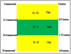
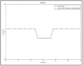
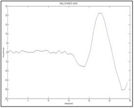
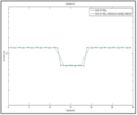
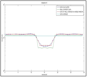
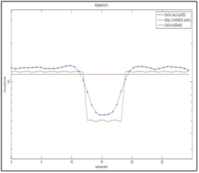
To test our computer code bul it up with expressions given above, we used the Ricker source wave function with a predominant frequency of 0.1 cycles/nanosecond, and is shown in Figure 3.The synthetic wave that simulates the wave recorded in the surface for the acquisition system (synthetic electromagnetic wave without noise) is shown in Figure 4, and is obtained from the convolution of the Ricker wave with the relative electrical permittivity of the geological model (Figure 1). In Figure 5 we present both the relative electric permittivity model (perturbation from the initial reference model) of the well, and the one obtained in a second step by means of a moving window average with 2 samples. These models were used to estimate the covariance matrix of the model, through the equations from (6) to (10). The calculated relative electrical permittivity data is made through the optimization method of the scaled conjugate gradient,² and the permittivity was initialized at a constant value equal to the average of the relative synthetic electrical permittivity data of well. The Figure 6shows the initialization data of the optimization algorithm (light blue), the synthetic data of real permittivity (line dark green, real synthetic data), the wellbore permittivity data averaged with the moving window (line red), and the calculated permittivity data (line dark blue)

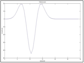
Figure 3 Source time function in terms of Ricker pulse, given in nanoseconds.

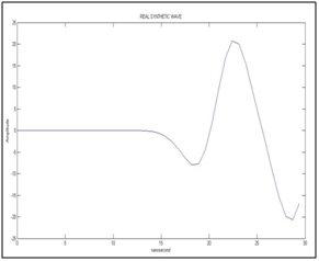
Figure 4 Synthetic “recorded” wave form (without noise) versus time in nanoseconds.

Figure 5 Relative electric permittivity in the well and its average made with a moving window that uses 2 samples, these are a function of nanosecond time.

Figure 6 Shows the initialization data of the optimization algorithm (light blue), the synthetic data of permittivity of the model (dark green, real synthetic data), the averaged relative electric permittivity of well in a mobile window (red ), and the calculated permittivity data (dark blue) for the synthetic electromagnetic wave without noise, all as a function of nanosecond time.

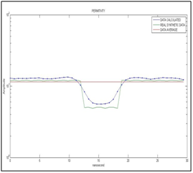
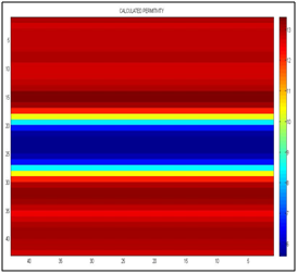
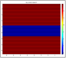
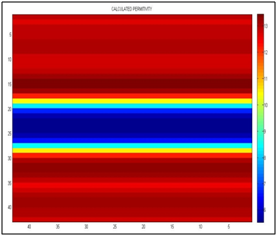
The initialization data of the optimization algorithm has a constant value of relative permittivity of 11.2, which is observed in Figure 7, and in which the red line shows the well permittivity data averaged with the moving window, and in color dark blue represents the calculated permittivity data for the synthetic electromagnetic wave without noise. When the program iterates, the initial data changes until the calculated data is obtained. In Figure 8 and 9, we show the real and calculated synthetic relative electrical permittivity, respectively, as also is observed for the geological model (Figure 1). Only 5 electric permittivity inversions were calculated and 38 equal to the previous ones were placed continuously (it is a means of parallel layers) to make
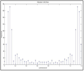
Figures 8-16 shown below. The synthetic wave that simulates the wave recorded at the top surface (synthetic electromagnetic wave with noise) is shown in Figure 10, and is obtained from the convolution of the Ricker wave with the relative electrical permittivity of the geological model (Figure 1), plus random Gaussian noise of amplitude 5% of the maximum amplitude of the synthetic wave without noise. For this model the sampling frequency is fs=1.43cycles/nanosecond and the maximum frequency of the synthetic wave (with noise) recorded on the surface is f_max=0.6cycles/nanosecond, which complies with the Nyquist sampling theorem. There is an aliasing lower than 5% in the region of the frequency of 0.6 cycles per nanosecond, therefore it is considered optimal to comply with the sampling theorem of Nyquist, see Figure 11.

The stopping criterion is taken when the gradient of the function target is minor that the number of observations (variables), also can be when:

${\left\{d_{obs}-g \left(\overrightarrow{Z}\right)\right\}}^T{C}_{dat}^{-1}\left\{d_{obs}-g\left(\overrightarrow{Z}\right)\right\} \le N$ (17)

Where N is the number of observations.

Figure 7 Shows the calculated permittivity data (dark blue line) for the synthetic electromagnetic wave without noise, real synthetic permittivity (dark green line) and average permittivity (the initialization data of the optimization algorithm; red line). The scale of the vertical axis is in logarithmic.

Figure 8 It shows the real synthetic permittivity, the left vertical axis must be multiplied by 0.7 for that of the scale in nanoseconds, and the horizontal axis is separated by centimeters.

Figure 9 It shows the calculated permittivity, the left vertical axis must be multiplied by 0.7 for that of the scale in nanoseconds, and the horizontal axis is separated by centimeters. We can see the interfaces between clay-sand at 12 nanosecond and sand-clay at 18 nanosecond.

Figure 10 Shows the synthetic wave recorded by the geophone (with noise) versus time in nanoseconds.

Figure 11 Shows the module of the fast Fourier transform versus the frequency in cycles/nanoseconds for synthetic wave with noise.

Figure 12 Shows the relative electric permittivity of the well and its average made with a mobile window that uses 2 samples, these are a function of nanosecond time. The scale of the vertical axis is in logarithmic.

Figure 13 Shows the initialization data of the optimization algorithm (light blue), the synthetic data of real permittivity (dark green), the electric permittivity data averaged in a moving window (red ), and the calculated permittivity data (dark blue)for the synthetic electromagnetic wave with noise, all as a function of nanosecond time. The scale of the vertical axis is in logarithmic.

Figure 14 Shows the calculated permittivity data (dark blue line) for the synthetic electromagnetic wave with noise, real synthetic permittivity (dark green line) and average permittivity (red line). The scale of the vertical axis is in logarithmic.

Figure 15 It shows the real synthetic permittivity, the left vertical axis must be multiplied by 0.7 for that of the scale in nanoseconds, and the horizontal axis is separated by centimeters.

Figure 16 It shows the calculated permittivity, the left vertical axis must be multiplied by 0.7 for that of the scale in nanoseconds, and the horizontal axis is separated by centimeters. We can see the interfaces between clay-sand and sand-clay at 12 nanosecond and sand-clay at 18.5 nanosecond approximately.

The covariance matrix of the synthetic data is diagonal and its variance was chosen equal to one, while the covariance matrix of the model has a value of 0.5 on its diagonal, the latter being smaller which causes the permittivity calculated for the Synthetic wave with and without noise, fit fairly close to the electric permittivity of the averaged well produced by the moving window (this averaging is the center of the a priori probability density), and give acceptably close to the real synthetic permittivity. It is observed that the scaled conjugate gradient method works well for this type of optimization. It is observed that with this inversion technique the medium can be characterized, and if the complex component of the permittivity is calculated by some mathematical model, the characterization of the medium would be extended for other types of soil and frequencies. The RAM memory of the laptop is 2 GHz, and Intel Core Duo, the run took 170 minutes per trace. Generally speaking, higher performance requires more memory and more running time. In the future, the issue of running time can be further addressed by the distributed parallel algorithm or the GPU implementation.

None.

The author declares there is no conflict of interest.

1. Daniels D, Gunton D, Scott H. Introduction to subsurface radar. IEE Proceedings. 1998;135(4):278‒320.
2. Martin F Moller. A Scaled Conjugate Gradient Algorithm for Fast Supervised Learning. University of Aarhus, Neural Networks. 1993;6(4):525‒533.