Solar radiation is one of the most important climatic parameters that is involved in different environmental, hydrological, agricultural applications while not always measured at all weather stations due to the high equipment and maintenance cost. The objectives of this study were to evaluate the performance and accuracy of twenty temperature based solar radiation models at five weather stations (Alcalde, Fabian Garcia, Farmington, Leyendecker and Tucumcari) in New Mexico and to evaluate the impact of solar radiation prediction on the Penman-Monteith grass reference evapotranspiration (ETo) for the global period of 2009-2017. New constants of each model at each weather station were retrieved using the optimization procedure Solver in Excel that maximizes the Kling-Gupta Efficiency (KGE). The root mean squared error (RMSE), mean absolute error (MAE), mean bias error (MBE) and the Nash-Sutcliffe model efficiency coefficient (NSE) were used for model performance evaluation. The results showed that the Hargreaves and Samani (1982), improved by Allen 1995, Bristow-Campbell (1984), Hunt et al. (1998), Fan et al. (2018), Hassan et al. (2016), Samani (2000); Nage et al. (2018) 2 and the Richardson et al (2018) models were the most accurate and the best performing ones across all five research sites. The EL-Sabaii, Ert Yal and Clemence models showed the poorest performance at all five stations. The evaluation of the impact of the predicted solar radiation on the Penman-Monteith ETo showed that predicted solar radiation had non-significant effect of the daily ETo with a regression slope varying from 0.978 to 1.022, RMSE from 0.24 to 0.48 mm/day, MAE from 0.15 to 0.31 mm/day and MBE from -0.03 to 0.09 mm/day. All solar radiation models showed best performance at Farmington and Tucumcari while they registered the poorest performance at Alcalde. The Student T-test revealed non-significant differences between the daily ETo using the measured solar radiation data set and the predicted solar radiation by each of the twenty solar radiation models at each weather station. The new models developed in this study could be used to estimate daily solar radiation across the semiarid environment of New Mexico for satisfactory estimation of ETo.

Keywords: solar radiation, prediction, reference evapotranspiration, semiarid climate

Solar radiation is the main source of available energy for different physical and physiological activities on the earth including crop growth and development, photosynthesis, evaporation, transpiration, snow melt, cloud formation, and different forms of energy transfer. Despite its importance, solar radiation measurement is tedious and  expensive in terms of equipment cost and maintenance in opposite to other climate variables such as air temperature, relative humidity, wind speed and precipitation.^1,2 As one of the most important climate variables, numerous studies have been conducted to develop models estimating solar radiation. As a result, different solar radiation models have been developed, evaluated and calibrated across the globe.^3‒11 Solar radiation models could be classified as temperature based, sunshine duration based, cloudiness and complex temperature - sunshine duration, temperature – precipitation, sunshine duration –precipitation or more complex models. Remote sensing and satellites are also used to retrieve solar radiation.¹² Fan et al.¹³ evaluated different temperature based solar radiation models. They concluded that the incorporation of daily precipitation and relative humidity within the temperature based models, improved the accuracy of the simple models for estimating solar radiation in the humid subtropical and tropical regions of south China. Quej et al.¹⁴ also reported that the complex models based on air temperature, air relative humidity, and precipitation gave  best performances compared to simple temperature based models. Recently, Feng et al.¹⁵ developed, evaluated and calibrated nineteen solar radiation models across 96 weather stations in China and reported  that calibration improved the prediction accuracy of solar radiation with root mean squared error (RMSE) of 16.5% and daily mean absolute error (MAE) of 1.69MJm^-2. From cross comparison of 300 sunshine-based solar radiation models in Nagpur (India), Makade and Jamil¹⁶ had shown that these models when calibrated to the local conditions gave best estimation. While most of the developed models are able to predict the daily solar radiation, their accuracy varies with the climatic zones and the quality of the available meteorological data. Model calibration to the local climatic conditions usually improves the performance and the accuracy of the models.^13,15,17,18

Crop evapotranspiration (ETc) is an important parameter in hydrological, environmental and agricultural studies and plays a key role in designing and managing irrigation projects and water management under irrigated and rainfed agriculture. While crop ETc is directly measured with lysimeters, Bowen ratio energy balance system and Eddy covariance systems,^19‒21 it is also estimated by the indirect method using reference crop evapotranspiration (ETo) and crop coefficients as proposed by Jensen.^22‒24 Evapotranspiration is one of the largest components of the hydrological cycle and is expected to increase with the warming across the Southwestern United States.²⁴ Water resources are limited under semiarid regions similar to the Southwestern United States, the hottest and driest region in the United States with diminishing winter and spring precipitation and shifts in precipitation and reference evapotranspiration.^25‒28 This projection is mostly challenging regarding water resources management and planning when the human population is increasing along with the demand for food and an increasing competition among water users such as agricultural producers, industries, mines, communities, environmentalists and others. Prein et al.²⁹ indicated that the southwestern United States climate may be transitioning to a drier climate state leading to higher drought risk. To cope with the aforementioned climatic conditions and the future projection, accurate estimation of crop water use may be a priority for water management and planning under conservative agriculture. Reference evapotranspiration (ETo) is estimated by different methods from direct measurements with lysimeters and Eddy covariance system to indirect modeling using local climatic variables.^4,30‒37 Numerous ETo equations have been developed with different parameterizations. Their performance and adaptability vary throughout the globe and the Penman-Monteith equation is shown to be the most worldwide accurate under all types of climatic conditions.^34,38‒46 However, the number of climatic variables required by the Penman-Monteith equation is the most limiting constraint for its adoption under limited data conditions. As aforementioned, solar radiation is the most scared measured variable and the simulation of this variable could partly help overcome data limitation for the Penman-Monteith equation adoption to improve water management under changing climate. The objectives of the present study were to (1) evaluate the performance of the nineteen existing and one developed temperature based solar radiation models and (2) evaluate the impact of the predicted solar radiation estimates on the Penman-Monteith grass reference evapotranspiration as a case study in a semiarid climate of the state of New Mexico.

Study area

This study was conducted at five weather stations across New Mexico (USA): Alcade, Fabian-Garcia, Farmington, Leyendecker and Tucumcari for the period of 2009-2017. The geographical coordinates and the long term average climatic variables at each station are summarized in Table 1. Minimum temperature (T_min), maximum temperature (T_max), minimum relative humidity (RH_min), maximum relative humidity (RH_max), wind speed (u₂), and solar radiation (Rs) were collected on the daily basis from automated weather stations installed by the New Mexico Climate Center. The time series data were check for quality control following the methodology described by Allen et al.³⁴

Empirical methods to estimate daily solar radiation

Twenty empirical methods were used to estimate daily solar radiation in this research. One simple equation with any exponet (equation 21) was developped in this study to facilited solar radiation estimation with very basic tools as most of the ranchers across the study area are within the upper age class and have limited accress to the highly efficiency estimation tools. The selected models are:

Hargreaves and Samani³ and Allen⁴⁷

$Rs=a*{\left(\frac{p}{101.3}\right)}^{0.5}*�T^{0.5}*Ro$       (1)

$p=101.3*{\left(\frac{293-0.0065 Z}{293}\right)}^{5.26}$       (2)

Bristow-Campbell⁵

$Rs=a*\left(1-e^{b{\left(�T\right)}^{0.5}}\right)*Ro$      (3)

Hargreaves and Samani⁴

$Rs=a*�T^{0.5}*Ro$      (4)

Clemence⁴⁸

Rs= a  (b*Ro*T+c T_max T+d T+e)      (5)

$Rs=a*\left(b*RoT+c*Tmax*T+d*T+e\right)$     (6)

Hunt et al.¹⁰

$Rs=a*Ro*�T^{0.5}+b$        (7)

Ertekin-Yaldiz⁴⁹

$Rs=a+b*Ro+c*T$         (8)

Samani⁶

$Rs=Ro*\left(a* �T^{0.5}+b* �T^{1.5}+c*�T^{2.5}\right)$       (9)

Annandale et al.⁵⁰

$Rs=a*\left(1+2.7*{10}^{-5}*Z*�T^{0.5}\right)*Ro$    (10)

Chen et al.⁹ named Chen1

$Rs=Ro*\left(a*ln\left(\Delta T\right)+b\right)$   (11)

Chen et al.⁹ named Chen2 Hargreaves et al.⁵¹

$Rs=Ro*\left(a*�T^{0.5}+b\right)$    (12)

El-Sebaii et al.⁵²

Rs=(a+b*T+c*RH)*Ro    (13)

Benghanem and Mellit.⁵³

Rs=a*Ro*∆T^0.25+b     (14)

Hassan et al.⁸

$Rs=Ro*\left(a+b*T\right)*�T^C$     (15)

Rao et al.⁵⁴

$Rs=a*Ro*e^{b{\left(�T\right)}^{0.5}}$     (16)

Jahani et al.¹

$Rs=Ro*(a+b*�T+c*{\left(�T\right)}^2+d*{\left(�T\right)}^3$      (17)

Fan et al.¹³

$Rs=Ro*(a+b*�T+c*{\left(�T\right)}^{0.25}+d*{\left(�T\right)}^{0.5}$      (18)

Nage et al.⁵⁵ named Nage1

$Rs=\left(a*�T^{0.7}*R{o}^{1.3}+b\right)*Ro$      (19)

Nage et al.⁵⁵ named Nage2

$Rs=\left(a+b*�T^{0.5}+c*\ln \left(�T\right)\right)*Ro$     (20)

Richardson et al.⁵⁶

$Rs=a* �T^b*Ro$     (21)

Djaman et al.

$Rs=\left(a+b*�T\right)*Ro$     (22)

where Ro=the daily extraterrestrial solar radiation (MJm^-2) determinded following the procedure described by Allen et al.³⁴; 𝞓T=(Tmax-Tmin); T=(Tmax+Tmin)/2; T, 𝞓T, Tmax and Tmin in ^oC; RH=mean relative humidity (%); Z=station altitude (m); a, b, c, d and e are dimenssionless empirical constants to be determined during the calibration process.

Penman-monteith reference evapotranspiration

Daily grass-reference evapotranspiration was computed using the standardized ASCE form of the Penman–Monteith equation³⁸ (Equation 22):

$ETo=\frac{0.408 � \left(Rn-G\right) + \frac{900\gamma u2}{T+273} \left(es-ea\right)}{�+\gamma \left(1+0.34 u2\right)}$     (23)

where, ETo is reference evapotranspiration (mm/day), Δ is the slope of saturation vapor pressure versus air temperature curve (kPa^oC^-1), Rn=net radiation at the crop surface (MJ m^-2 d^-1), G=soil heat flux density at the soil surface (MJ m^-2 d^-1), Tmax and Tmin are maximum and minimum air temperature (⁰C), T=mean daily air temperature at 1.5-2.5m height (^oC), u₂=mean daily wind speed at 2m height (m s^-1), es=the saturation vapor pressure (kPa), ea=the actual vapor pressure (kPa), es-ea=saturation vapor pressure deficit (kPa), γ=psychrometric constant (kPa ^oC^-1),. Rs=solar radiation (MJ m^-2 d^-1). All parameters necessary for computing ETo were computed according to the procedure developed in FAO-56 by Allen et al.³⁴ 

Calibration of the daily solar irradiation models

The original solar radiation equations were calibrated to the local semiarid and dry climatic conditions of each location. These solar radiation equations were calibrated using the measured daily solar radiation data and the generalized reduced gradient method. This procedure allows iterations by changing the constants in the equations to create new equations for each location. The solver add-in Excel is a tool that was used to fit the original equations by minimizing the sum of the squared residuals. Multiple initial values were tested to ensure that the global minimum of the errors was found⁵⁷ and maximum value of the Kling-Gupta efficiency (KGE)⁵⁸ was reached. For model evaluation, simple linear regression was used to compare the daily solar radiation estimates by the temperature based solar radiation models and the measured daily solar radiation at each weather station. The intercept of the regression line was forced to be zero. The more accurate the solar radiation equation is the more the regression slope and the coefficient of determination are close to unity. The coefficient of determination R², the Kling-Gupta efficiency (KGE),⁵⁸ Root mean square error (RMSE), Nash-Sutcliffe model efficiency coefficient (NSE), and the mean absolute error (MAE)¹⁸ were also used for model evaluation. The objective function was to maximize R² and KGE (the higher R² and KGE are, the better is the simulation process) and to minimize RMSE, MAE, NSE, and MBE. The sign of the MBE indicates overestimation of the solar radiation estimates (MBE>0) or underestimation of the solar radiation estimates (MBE<0). 

Evaluation of the impact of solar radiation simulated by empirical models on the Penman-Monteith reference evapotranspiration estimates

The measured and predicted daily solar radiation were interchanged in combination with all other required weather variables (Tmax, Tmin, RHmax, RHmin and U₂) to estimate daily ETo under both conditions. The Penman-Monteith ETo (ETo-PM-meas) estimates using the measured daily solar radiation was compared to the one using the predicted daily solar radiation by the temperature based solar radiation models (ETo-PM-pred) using simple linear regression with the intercept forced to be zero. The evaluation criteria used for solar radiation models evaluation are also used for the evaluation of the impact of the solar radiation models on the Penman-Monteith reference evapotranspiration estimates. In addition, Student T-test was used to compare the ETo-PM-meas and ETo-PM-pred across all models and weather stations to determine any significant difference between the original ETo estimates and the predicted ETo values using predicted solar radiation values at 95% level of confidence.

Calibration and evaluation of the solar radiation models

The selected solar radiation models showed different performance and accuracy at each of the five weather stations under this study (Figures 1‒3). The best fitting constants that optimized the daily solar radiation estimation at each weather station and for each of the selected models are summarized in Table 2. The boxplots of the performance criteria are presented in Figure 1. The Kling-Gupta efficiency (KGE) varied with model and locations and ranged from 0.69 to 0.91 (Figure 2). The best model at all five weather stations combined with the greatest accuracy was the Hassan’s model obtaining an average medium KGE value of 0.90 followed by Fan et al., Bist Camp, Samani and Cichar and the models. The lowest KGE values were obtained for the Benghamen, EsSebaii, Ert Yal and Clemence models (Figure 1). Clemence showed the lowest medium KGE value of 0.79. All models performed better at Farmington followed by Tucumcari, Fabian Garcia and Alcalde (Figure 2). Considering average KGE value, Hassan’s model was the best performing model (KGE value=0.89) and Benghamen and Clemence are the least performing models with average KGE value of 0.80.

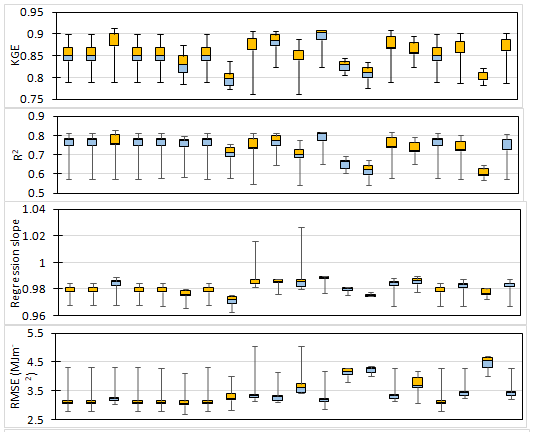
Figure 1 Boxplots of the statistics evaluation criteria for solar radiation models at five weather stations (pooled) in New Mexico.

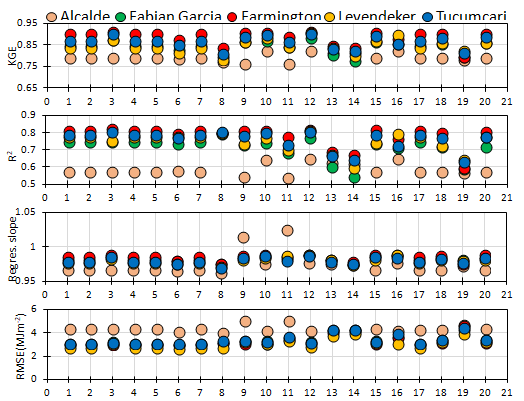
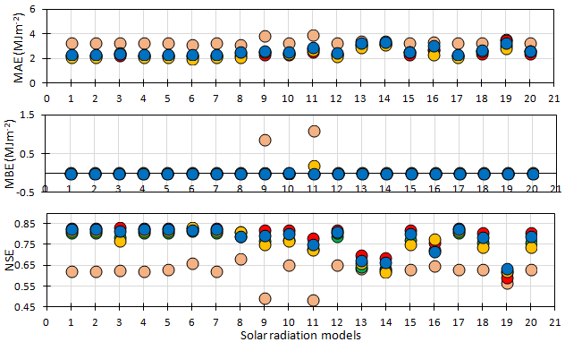
Figure 2 KGE, R², regression slope, root mean squared error (RMSE), mean bias error (MBE), mean absolute error (MAE) and Nash-Sutcliffe model efficiency coefficient (NSE) between the measured and the predicted daily solar radiation using different solar radiation models at Alcalde. Fabian Garcia, Farmington, Leyendecker, and Tucumcari. The order of the solar radiation models 1, 2, 3…, 20 is the same as in Figure 1.

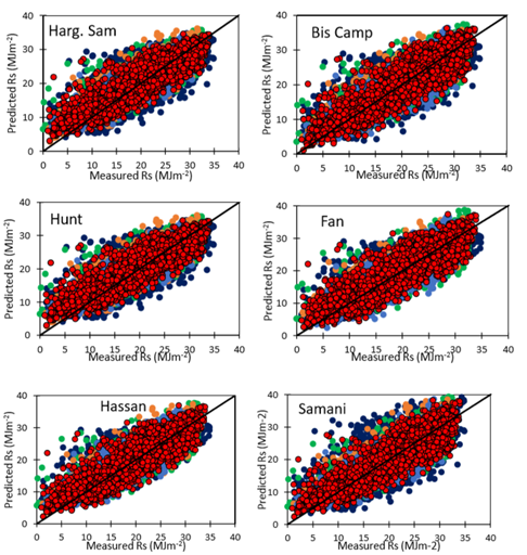
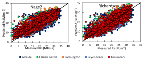
Figure 3 Regression plotting between the measured and the predicted daily solar radiation by the best eight solar radiation models at Alcalde. Fabian Garcia, Farmington, Leyendecker, and Tucumcari.

The coefficient of determination of the regression between the measured and the predicted daily solar radiation estimates was dependent on the model. The boxplots of R² showed that most of the models obtained moderately high values except for the El-Sebaii, Ert Yal and Clemence models with R² values lower than 0.70. However, when most models showed boxplot high median R² value, the minimum R² values were quite low between 0.54 and 0.58. All models showed the highest R² values at Farmington weather station and the lowest R² values at Alcalde weather station (Figure 2). The highest and the lowest values of R² were showed by Bist Camp model and Johani model, respectively (Figure 1).

High regression slope between the measured and the predicted daily solar radiation values were obtained and varied from 0.96 and 1.03 (Figure 2). The boxplots showed that the regression slope values are lower than unity for most of the models with the boxes below the y=1 line while Samani and Johani showed maximum value greater than unity, indicating solar radiation overestimation at Alcalde (Figure 2). Hassan’s model was still the best performing model and the Berghamen’s model showed the lowest regression slope. All models showed the lowest regression slope at Alcalde except Samani and Johani models.

Root mean square error (RMSE) of the predicted daily solar radiation estimates varied within a wide range between 2.67 and 5.71MJm^-2 as shown in Figure 2. RMSEvalues were concentrated between 3 and 3.5MJm^-2 for most of the models except for Johani, El Sebaii, Ert-Yal, Nage1 and Clemence models which showed higher RMSE values (Figure 1). Overall, models showed the lowest RMSE values at Leyendecker while they showed the highest RMSE values at Alcalde and the intermediate RMSE values were obtained at Farmington and Tucumcari. The Samani and Johani models showed the highest RMSE at Alcalde and the lowest RMSE value was shown by Chen2 at Leyendecker (Figure 2).

The mean absolute error (MAE) ranged from 2.36 to 3.87MJm^-2 (Figure 2). The boxplots showed low MAE with most of the boxes within the range of 2.2–2.7 (Figure 1). Johani, El-Sebaii, Ert YAl, Nage1 and Clemence models showed great MAE while all models showed the maximum MAE greater than 3MJm^-2 at Alcalde (Figure 1). Similar to the RMSE, the highest MAE values were obtained at Alcalde and the lowest MAE were registered at Leyendecker (Figure 2). Overall, the model Chen2 showed the lowest MAE value of 2.40MJm^-2 and the highest MAE value of 3.26MJm^-2 was obtained by Clemence model. The mean bias error (MBE) were quite low and ranged between -0.01 and 1.07MJm^-2. Only Samani and Johani models showed MBE values of 0.85 and 1.08MJm^-2 at Alcalde, respectively, and Johani showed MBE value of 0.18MJm^-2 at Leyendecker as the highest MBE values (Figure 2). The Nash-Sutcliffe model efficiency coefficient (NSE) varied from 0.49 to 0.83 while most of the NSE boxplots are within the range of 0.75-0.83. El-Sebaii, Ert Yal and Clemence models have the boxes below 0.7 and the Samani and Johani models showed the lowest values of NSE (Figure 2). The lowest values of the NSE recorded at Alcalde for all models and very clustered values were observed at Fabien Garcia, Farmington, Leyendecker and Tucumcari (Figure 2).

From the combination of all the evaluation criteria, the most accurate and best performing solar radiation models across New Mexico were: Hargreaves and Samani³ improved by Allen,⁴⁷ Bristow-Campbell,⁵ Hunt et al.,¹⁰ Fan et al.,¹³ Hassan et al.,⁸ Samani;⁶ Nage et al.⁵⁵ 2, Richardson et al.⁵⁶ Daily solar radiation estimates by these top eight best performing models were plotted against the mesured daily solar radiation at all five weather stations and satisfactory superposed as shown in Figure 3. Threfore, these models could be used to simulated daily solar radiation using air maximum, minimum and average temparature in New Mexico. The results of this study are in agreement with Jamil et al.⁵⁹ who had predicted solar radiation from the temperature extremes using 33 different models in India. The most accurate and best performing models according to their study were three models of Hassan et al.⁸ One the Hassan’s model was shown as one of the most accurate models across the semiarid environment of New Mexico. Bristow-Campbell and Hargreaves and Samani models were evaluated with satisfactory in Chile by Meza and Varas.⁶⁰ Bandyopadhyay et al.⁶¹ found that the Hargreaves model was the best model for estimating solar radiation from air maximum and minimum temperatures while Tabari et al.⁶² reported one of Chen models and the improved Hargreaves model by Allen⁴⁷ to be the best performing ones across the cool semiarid climate while the same models in addition to Annandale model performed better in the arid region in Iran. They indicated that Ertekin-Yaldiz model showed better performance in the cool semiarid environment than other climatic regions. Hargreaves and Samani model was used to predict solar radiation in Spain with high R² value of 0.87.⁶³ Li et al.⁶⁴ reported that the modified Hargreaves and Chen models performed better than the original models. Valiantzas⁶⁵ modified the Hargreaves-Samani model and proposed a new model which performed well using data from California, Arizona in the Southwest United States. Estévez et al.⁶⁶ and Grillone et al.⁶⁷ had shown the applicability of different solar radiation models after recalibration to local conditions. While diverse results were obtained from solar radiation models evaluation under different climatic conditions across the globe, the performance of these models is improved by site specific calibration and model choice may consider the climatic conditions under which the models were developed and the available data should be check for data quality control.

Impact of the predicted solar radiation on the Penman-Monteith reference evapotranspiration

Daily grass reference evapotranspiration was estimated by the Penman-Monteith equation using the measured solar radiation and the predicted solar radiation by the selected solar radiation models. The impact of the solar radiation prediction accuracy on the performance of the Penman-Monteith equation was drawn and the results showed that solar radiation prediction accuracy had a little effect on the reference evapotranspiration estimates. The coefficient of determination of the simple linear regression line between the ETo-PM-meas and the ETo-PM-pred varied with locations and solar radiation model used. It ranged from 0.94 to 0.99 and the highest R² value were observed at Farmington and Tucumcari for all solar radiation models. The lowest R² values were registered at Alcalde (Figure 4).

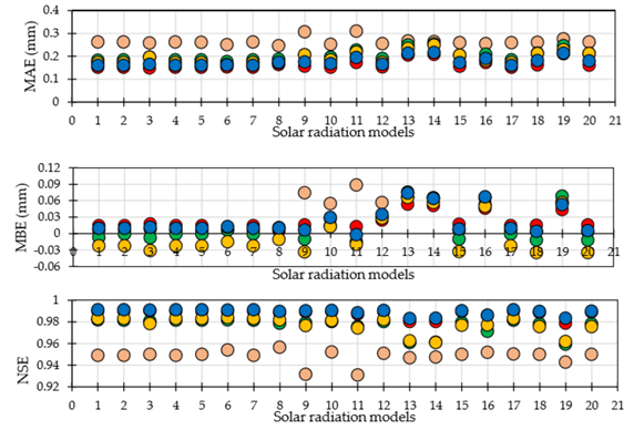
Figure 4 R2, regression slope, root mean squared error (RMSE), mean bias error (MBE), and mean absolute error (MAE) and Nash-Sutcliffe model efficiency coefficient (NSE) between the original and the predicted daily reference evapotranspiration using predicted daily solar radiation with the different models at Alcalde, Fabian Garcia, Farmington, Leyendecker, and Tucumcari. The order of the solar radiation models 1, 2, 3…, 20 is the same as in Figure 1.

The regression slope varied from 0.978 to 1.022 showing the relatively high correlation between the two sources of ETo estimates. Slight overestimation of ETo was mostly observed at Farmington with a regression slope greater than unity however, the highest ETo overestimation was obtained at Alcalde when daily solar radiation was predicted by the Samani, Fan, El-Sabaii, and Johani models. Daily ETo was systematically overestimated at all five stations when the solar radiation was predicted by the Hassan, El Sebaii, Ert Yal, Nage1 and Clemence models (Figure 4). Overall, the lowest regression slope was obtained at Leyendecker and the maximum ETo overestimation and underestimation equal to 2.2% seems to be reasonable.

Low RMSE of ETo estimates were obtained and varied from 0.24 to 0.48mm/day with the highest RMSE observed at the Alcalde (Figure 4). Similarly, very low MAE and MBE values were observed and ranged from 0.15 to 0.31mm/day (Figure 4) and from -0.03 to 0.09mm/day (Figure 4), respectively. The highest MAE values were obtained at Alcalde and the lowest values were obtained at Farmington (Figure 4) while the lowest MBE values were obtained at Leyendecker and the highest MBE value were not systematically obtained at only one station. Solar radiation predicted by Samani, Fan et al, Hassan, El-Sebaii, ERt Yal, Nage1 and Clemence models are sources of the high MBE of the predicted ETo values. The overall performance of the solar radiation models showed non-significant impact on the ETo estimates and the Nash-Sutcliffe model efficiency coefficient (NSE) values were quite high and varied from 0.93 to 0.99 with the lowest values of NSE observed at Alcalde and the highest NSE values observed at Farmington and Tucumcari across all solar radiation models (Figure 4). NSE values averaged 0.95, 0.98. 0.99, 0.98 and 0.99 at Alcalde, Fabian Garcia, Farmington, Leyendecker and Tucumcari, respectively.

The Student T-test revealed non-significant differences between the original and the predicted ETo values across all five weather stations using any of the 20solar radiation models. Consequently, the different solar radiation models have non-significant impact on estimating daily grass reference evapotranspiration. The good fitness of the predicted ETo versus the observed ETo estimates is shown in Figure 5 presenting the impact of the best eight solar radiation models on ETo estimates. These results are in agreement with Tabari et al.⁶² and Bandyopadhyay et al.⁶¹ who reported that the solar radiation prediction model choice had a little impact on the reference evapotranspiration estimates. Tabari et al.⁶² reported no noticeable improvement in ETo estimates when daily solar radiation data was predicted by the Hargreaves-Samani, Allen, Samani, Annandale, Chen and Ertekin-Yaldiz models with Penman-Monteith ETo deviation range between from -2.16 to 1.40mm between the original and the calibrated solar radiation.

Figure 5 Regression plotting between the original Penman-Monteith ETo with the measured solar radiation and the predicted Penman-Monteith ETo with the predicted solar radiation by the best eight solar radiation models at Alcalde, Fabian Garcia, Farmington, Leyendecker, and Tucumcari.

Performance and accuracy of twenty temperature based solar radiation models were evaluated at five weather stations in New Mexico for the global period of 2009-2017 using the optimization procedure Solver in Excel which maximized the Kling-Gupta Efficiency. The results showed that the Hargreaves and Samani³ improved by Allen,⁴⁷ Bristow-Campbell,⁵ Hunt et al.,¹⁰ Fan et al.,¹³ Hassan et al.,⁸ Samani,⁶ Nage⁵⁵ 2, and Richardson⁵⁶ models were the most accurate and the best performing ones across all research sites with the highest Kling-Gupta Efficiency, the root mean squared error (RMSE), mean absolute error (MAE), mean bias error (MBE), and the Nash-Sutcliffe model efficiency coefficient. The evaluation of the impact of the predicted solar radiation on the Penman-Monteith reference evapotranspiration showed that the predicted solar radiation had non-significant effect of the daily reference evapotranspiration with regression slopes varying from 0.978 to 1.022, RMSE from 0.24 to 0.48mm/day, MAE from 0.15 to 0.31mm/day and MBE from -0.03 to 0.09mm/day. These best performing solar radiation models could be considered as the alternatives for estimating daily solar radiation across New Mexico when solar radiation is missing and for predicting daily reference evapotranspiration across the study area.

We completed this work with the support of New Mexico State University (NMSU) and the Agricultural Science Center at Farmington and all the staff.

The authors declare no conflict of interest.

None.

1. Jahani B, Dinpashoh Y, Raisi Nafchi A. Evaluation and development of empirical models for estimating daily solar radiation. Renew. Sustain. Energy Rev. 2017;73:878–891.
2. Fan J, Wu L, Zhang F, et al. Evaluation and development of empirical models for estimating daily and monthly mean daily diffuse horizontal solar radiation for different climatic regions of China. Renew Sustain. Energy Rev. 2019;105:168–186.
3. Hargreaves G, Samani ZA. Estimating Potential Evapotranspiration. J Irrig Drain Div ASCE. 1982;08:225–230.
4. Hargreaves GH, Samani ZA. Reference crop evapotranspiration from temperature. Applied Engineering in Agriculture. 1985;1(2):96–99.
5. Bristow KL, Campbell GS. On the relationship between incoming solar radiation and daily maximum and minimum temperature. Agricultural and Forest Meteorology. 1984;31(2):159–166.
6. Samani Z. Estimating Solar Radiation and Evapotranspiration Using Minimum Climatological Data. Journal of Irrigation and Drainage Engineering. 2000;126(4):265–267.
7. Almorox J, ChiquinquiráHontoria F. Global solar radiation estimation using sunshine duration in Spain. Energy Conversion and Management. 2004;45(9–10):1529–1535.
8. Hassan GE, Youssef ME, Mohamed ZE, et al. New Temperature–based Models for Predicting Global Solar Radiation. Applied Energy. 2016;179:437–450.
9. Chen R, Ersi K, Yang J, et al. Validation of five global radiation models with measured daily data in China. Energy Convers. Manag. 2004;45(11):1759–1769.
10. Hunt LA, Kuchar L, Swanton CJ. Estimation of solar radiation for use in crop modelling. Agricultural and Forest Meteorology. 1998;91(3):293–300.
11. Bayrakçi HC, Demircan C, Keçebacs A. The development of empirical models for estimating global solar radiation on horizontal surface: a case study. Renewable and Sustainable Energy Reviews. 2018;81(2):2771–2782.
12. Xu X, Du H, Zhou G, et al. A method for daily global solar radiation estimation from two instantaneous values using MODIS atmospheric products. Energy. 2016;111:117e25.
13. Fan J, Chen B, Wu L, et al. Evaluation and development of temperature–based empirical models for estimating daily global solar radiation in humid regions. Energy. 2018;144:903–914.
14. Quej VH, Almorox J, Ibrakhimov M, et al. Empirical models for estimating daily global solar radiation in Yucatán Peninsula, Mexico. Energy Convers. Manage. 2016;110:448–456.
15. Feng Y, Hao W, Li H, et al. Machine learning models to quantify and map daily global solar radiation and photovoltaic power. Renew Sustain Energy Rev. 2020;118:109393.
16. Makade RG, Jamil B. Statistical analysis of sunshine based global solar radiation (GSR) models for tropical wet and dry climatic Region in Nagpur, India: a case study. Renew Sustain Energy Rev. 2018;87:22–43.
17. Djaman K, Balde AB, Sow A, et al. Evaluation of sixteen reference evapotranspiration methods under sahelian conditions in the Senegal River Valley. J Hydro: Reg Stud. 2015;3:139–159.
18. Djaman K, O’Neill M, Diop L, et al. Evaluation of the Penman–Monteith and other 34 reference evapotranspiration equations under limited data in a semiarid dry climate. Theoretical and Applied Climatology. 2018;137(1–2):729–743.
19. Zitouna–Chebbi R, Prévot L, Chakhar A, et al. Observing Actual Evapotranspiration from Flux Tower Eddy Covariance Measurements within a Hilly Watershed: Case Study of the Kamech Site, Cap Bon Peninsula, Tunisia. Atmosphere. 2018;9:68.
20. Irmak S, Payero JO, Kilic A, et al. On the magnitude and dynamics of eddy covariance residual energy (energy closure) from a subsurface drip–irrigated maize field during growing and non–growing (dormant) seasons. Irrigation Science. 2014;32:471–483.
21. Liu B, Yuanlai C, Yuanzhi S, et al. Comparison of evapotranspiration measurements between eddy covariance and lysimeters in paddy fields under alternate wetting and drying irrigation. Paddy Water Environ. 2019;17:725.
22. Jensen ME. Water consumption by agricultural plants. In Water Deficits and Plant Growth. In: Kozlowski TT, Editors. Academic Press: New York: NY, USA. 1968;2:1–22.
23. Djaman K, Tabari H, Balde AB, et al. Analyses, calibration and validation of evapotranspiration models to predict grass reference evapotranspiration in the Senegal River Delta. Journal of Hydrology: Regional Studies. 2016;8:82–94.
24. Djaman K, O’Neill M, Owen CK, et al. Crop evapotranspiration, irrigation water requirement and water productivity of maize from meteorological data under semiarid climate. Water. 2018;10:405.
25. Archer SR, Predick KI. Climate change and ecosystems of the southwestern United States. Rangelands. 2008;30:23–28.
26. Cayan D, Tyree M, Kunkel K, et al. Future climate: Projected average. In Assessment of Climate Change in the Southwest United States: A Report Prepared for the National Climate Assessment. In: Garfin G, et al, Editors. Southwest Climate Alliance: Washington, DC, USA. 2013;101–125.
27. Garfin G, Franco G, Blanco H, et al. Southwest Climate Change Impacts in the United States: The Third National Climate Assessment. In U.S. Global Change Research Program. In: Melillo JM, Richmond TC, Yohe GW, Editors. The U.S. Government Printing Office, Washington, DC, USA. 2014;462–486.
28. Dettinger M, Udall B, Georgakakos A. Western water and climate change. Ecological Applications. 2015;25(8):2069–2093.
29. Prein AF, Holland GJ, Rasmussen RM, et al. Running dry: The US Southwest’s drift into a drier climate state. Geophys Res Lett, 2016;43(3):1272–1279.
30. Thornthwaite CW. An approach towards a rational classification of climate. Geogr Revue. 1948;38(1):55–94.
31. Turc L. Water requirements assessment of irrigation, potential evapotranspiration: simplified and updated climatic formula. Annales Agronomiques. 1961;12:13–49.
32. Penman HL. Vegetation and hydrology. Soil Science. 1963;96:357.
33. Abtew W. Evapotranspiration measurements and modelling for three wetland systems in South Florida. J Am Water Resour. Assoc. 1996;32:465–473.
34. Allen RG, Pereira LS, Raes D, et al. Crop Evapotranspiration–Guidelines for computing crop water requirements–FAO. Irrigation and Drainage paper 56. FAO, Rome; 1998.
35. Irmak S, Irmak A, Jones JW. Solar and net radiation–based equations to estimate reference evapotranspiration in humid climates. Journal of Irrigation and Drainage Engineering. 2003;129:336–347.
36. Trajkovic S. Hargreaves versus Penman–Monteith under humid conditions. Journal of Irrigation and Drainage Engineering. 2007;133(1):38–42.
37. Valiantzas JD. Simplified reference evapotranspiration formula using an empirical impact factor for penman’s aerodynamic term. Journal of Irrigation and Drainage Engineering. 2013;18:108–114.
38. ASCE–EWRI. The ASCE standardized reference evapotranspiration equation. In: Allen RG, Walter IA, Elliot RL, et al. Editors. Environmental and Water Resources Institute (EWRI) of the American Society of Civil. Engineers, ASCE, Standardization of Reference Evapotranspiration Task Committee Final Report; 2005. 213pp.
39. López–Urrea R, Martín de Santa Olalla F, Fabeiro C, et al. Testing evapotranspiration equations using lysimeter observations in a semiarid climate. Agricultural Water Management. 2006;85(1-2):15–26.
40. Bodner G, Loiskand W, Kaulm H. Cover crop evapotranspiration under semi–arid conditions using FAO dual crop coefficient method with water stress compensation. Agricultural Water Management. 2007;93(3):85–98.            
41. Jabloun M, Sahli A. Evaluation of FAO–56 methodology for estimating reference evapotranspiration using limited climatic data application to Tunisia. Agricultural Water Management. 2008;95(6):707–715.
42. Irmak S, Irmak A, Howell TA, et al. Variability analyses of alfalfa–reference to grass–reference evapotranspiration ratios in growing and dormant seasons. Journal of Irrigation and Drainage Engineering. 2008;134:147–159.
43. Xing Z, Chow L, Meng F, et al. Testing reference evapotranspiration estimation methods using evaporation pan and modeling in maritime region of Canada. Journal of Irrigation and Drainage Engineering. 2008;134(4):417–424.
44. Trajkovic S, Kolakovic S. Evaluation of reference evapotranspiration equations under humid conditions. Water Resour Manag. 2009;23(14):3057–3067.
45. Tabari H, Grismer M, Trajkovic S. Comparative analysis of 31 reference evapotranspiration methods under humid conditions. Irrigation Science. 2011;31:107–117.
46. Xystrakis F, Matzarakis A. Evaluation of 13 empirical reference potential evapotranspiration equations on the island of Crete in southern Greece. J Irrig Drain Eng. 2011;137(4):211–222.
47. Allen RG. Evaluation procedures for estimating mean monthly solar radiation from air temperature. Rome: United Nations Food and Agricultural Organization (FAO). 1995.
48. Clemence BSE. An attempt at estimating solar radiation at South African sites which measure air temperature only. South African Journal of Plant and Soil. 1992;9(1):40–42.
49. Ertekin C, Yaldiz O. Estimation of monthly average daily global radiation on horizontal surface for Antalia, Turkey. Renewable Energy. 1999;17(1):95–102.
50. Annandale JG, Jovanic NZ, Benade N, et al. Software for missing data error analysis of Penman–Monteith reference evapotranspiration. Irrigation Science. 2002;21:57–67.
51. Hargreaves LG, Hargreaves GH, Riley JP. Irrigation Water Requirements for Senegal River Basin. J Irrig Drain Eng. 1985;111(3):265–275.
52. El–Sebaii AA, Al–Ghamdi AA, Al–Hazmi FS, et al. Estimation of global solar radiation on horizontal surfaces in Jeddah, Saudi Arabia. Energy Policy. 2009;37(9):3645–3649.
53. Benghanem M, Mellit A. A simplified calibrated model for estimating daily global solar radiation in Madinah, Saudi Arabia. Theor Appl Climatol. 2014;115:197–e205.
54. Siva Krishna Rao KDV, Premalatha M, Naveen C. Models for forecasting monthly mean daily global solar radiation from in–situ measurements: Application in Tropical Climate, India. Urban Clim. 2017;24:921–939.
55. Nage GD. Estimation of Monthly Average Daily Solar Radiation from Meteorological Parameters: Sunshine Hours and Measured Temperature in Tepi, Ethiopia. International Journal of Energy Environmental Science. 2018;3(1):19–26.
56. Richardson CW. Stochastic simulation of daily precipitation, temperature, and solar radiation. Water Resour Res. 2018;17(1):182–190.
57. Bogawski P, Bednorz E. Comparison and validation of selected evapotranspiration models for conditions in Poland (Central Europe). Water Resour Manag. 2014;28(14):5021–5038.
58. Gupta HV, Kling H, Yilmaz KK, et al. Decomposition of the mean squared error and NSE performance criteria: implications for improving hydrological modelling. Journal of Hydrology. 2009;377(1-2):80–91.
59. Jamil B, Irshad K, Algahtani A, et al. On the calibration and applicability of global solar radiation models based on temperature extremities in India. Environmental Progress & Sustainable Energy. 2019;39(1).
60. Meza FVE, Varas E. Estimation of mean monthly solarglobal radiation as a function of temperature. Agricultural and Forest Meteorology. 2000;100(2-3):231–241.
61. Bandyopadhyay A, Bhadra A, Raghuwanshi NS, et al. Estimation of monthly solar radiation from measured air temperature extremes. Agricultural and Forest Meteorology. 2008;148(11):1707–1718.
62. Tabari H, Hosseinzadehtalaei P, Willems P, et al. Validation and calibration of solar radiation equations for estimating daily reference evapotranspiration at cool semi–arid and arid locations. Hydrological Sciences Journal. 2016;61(3):610–619.
63. Almorox J. Estimating global solar radiation from common meteorological data in Aranjuez, Spain. Turkish Journal of Physics. 2011;35:53–64.
64. Li H, Cao F, Wang X, et al. A temperature–based model for estimating monthly average daily global solar radiation in China. Scientific World Journal. 2014;128754.
65. Valiantzas DJ. Temperature–and humidity–based simplified Penman’s ET0 formulae. Comparisons with temperature–based Hargreaves–Samani and other methodologies. Agricultural Water Management. 2018;208:326–334.
66. Estevez J, Padilla FLM, Gavilan P. Evaluation and regional calibration of solar radiation prediction models in southern Spain. Journal of Irrigation and Drainage Engineering. 2012;138(10):868–879.
67. Grillone G, Agnese C, D’Asaro F. Estimation of Daily Solar Radiation from Measured Air Temperature Extremes in the Mid–Mediterranean Area. Journal of Irrigation and Drainage Engineering. 2012;138(10).