This paper deals with the analysis of the SOI and EQSOI series and their statistical properties, focussing in particular in their cyclical pattern and its persistence across time. For this purpose, a long memory model was used that is characterized because the spectral density function is unbounded at a frequency away from zero. Our results indicate that the two series display a long memory pattern, with the order of integration in the interval (0, 0.5) and the length of the cycles ranging between three and four years.

Keywords: SOI; EQSOI; cycles; fractional integration

The Southern Oscillation Index (SOI) is a normalized index based on the sea level pressure differences between Tahiti and Darwin in Australia. It measures air pressure fluctuations in large scale that takes place between the Western and Eastern tropical Pacific. Hence, SOI provides information about the intensity and development of El Niño and La Niña weather patterns. In general, a smooth behaviour of the SOI time series is associated with changes in ocean temperatures across the Eastern tropical Pacific. For instance, persistent negative values of the SOI are usually linked to abnormally warm in the Central and Eastern tropical Pacific Ocean and is typically known as El Niño episode. In contrast, sustained periods of positive SOI values correspond to La Niña and is associated with cooling of the Central and Eastern tropical Pacific Ocean.

It is worth mentioning that both Tahiti and Darwin are well South of the Equator and thus, the surface air pressure in these two locations may not be directly related to El Niño Southern Oscillation (ENSO). To sort out this issue, a new indicator has been proposed denominated the Equatorial SOI (EQSOI), which is calculated as the standardized anomaly of the difference between the area-average monthly sea level pressure in an area of the Eastern Equatorial Pacific (80°W - 130°W, 5°N - 5°S) and an area over Indonesia (90°E - 140°E, 5°N - 5°S). 

In this paper the persistence and cyclicity of these two well know series (SOI and EQSOI) were examined by using long memory models, and in particular, employed a fractionally integrated model where the singularity in the spectrum occurs at a frequency away from zero. The model is based on the Gegenbauer processes and the results indicate that the orders of integration of the series are in the interval (0, 0.5) displaying a long memory pattern. In addition, it is observed that cycles have a periodicity of about 37-42 periods (months), which is consistent with the literature that suggest oscillations between 3 and 7 years.

The rest of the paper is organized as follows: Section 2 briefly presents a review of the statistical modelling of the metric of the ENSO cycle throughout the SOI and EQSOI data; Section 3 describes the model used in the paper, while Section 4 is devoted to the methodology used and based on long memory processes. Section 4 displays the data and Section 5 contains the main empirical results. Finally, Section 6 concludes the paper.

The term El Niño/La Niña refers to the process of the irregular weather patterns associated with abnormally heating/cooling of the Central and Eastern tropical Pacific.¹ This phenomenon is related, among others, to the increased convection (e.g. changing Walker circulation), that alters cloudiness in the Central Pacific Ocean and causing a weaker or stronger than normal trade winds along the Pacific (Figure 1 (b), (c)).

It is well-established that the El Niño/La Niña phenomenon is linked to an oscillation of the surface air pressure between the Eastern and Western South Pacific, which is known as the Southern Oscillation (SO). The strength of this oscillating is measured by the Southern Oscillation Index (SOI), which is one of the key atmospheric indices for gauging the strength of the El Niño and La Niña events and their potential impacts on the Australian region (Bureau of Meteorology, Australian Government). SOI is a normalized index which is defined as the difference in the monthly surface air pressure between Tahiti (17º 40’S, 149º 25’ W) and Darwin (12º 27’ S, 130º 50’ E), as follows:

$SOI=\frac{\left(StardardizedTahiti-StardarizedDarwin\right)}{MSD},$

where,

$StardardizedTahiti=\frac{\left(ActualTahitiSLP-MeanTahitiSLP\right)}{StandardDeviationTahiti},$

and N is the number of months.

$StandardDeviationTahiti=\sqrt{{{\displaystyle \sum \left(actualTahitiSLP-meanTahitiSLP\right)}}^2/N},$

Where

$StandardDeviationDarwin=\sqrt{{{\displaystyle \sum \left(actualTahitiSLP-meanTahitiSLP\right)}}^2/N}$

And

$\begin{array}{l}MSD\left(MonthlyStandardDeviation\right)\\ ={\displaystyle \sum \frac{{\left(StandarizedTahiti-StandarizedDarwin\right)}^2}{N}}.\end{array}$

El Niño events are associated with negative values of the SOI (below about -8), while La Niña events are associated with positive SOI values (above about +8). The El Niño/La Niña Southern Oscillation (ENSO) is a quasi-periodic oceanic-atmospheric phenomenon with a typical periodicity of 3-7 years, and it is featured by three phases: neutral, El Niño and La Niña, as shown in Figure 1a, 1b and 1c, respectively (Bureau of Meteorology, Australian Government).

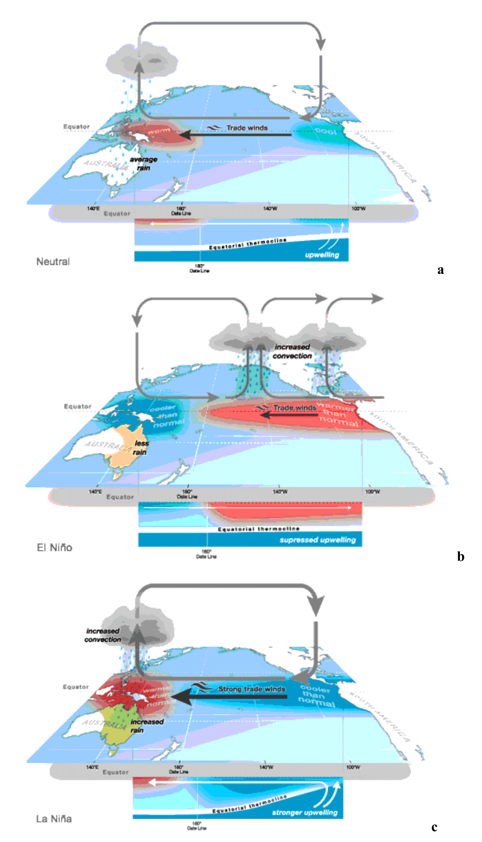
Figure 1 Phases of the ENSO: (a) Neutral, (b) El Niño, and (c) La Niña. [http://www.bom.gov.au/climate/enso/history/ln-2010-12/three-phases-of-ENSO.shtml]

In the neutral state (neither El Niño nor La Niña) (Figure 1a), trade winds blow across the surface of the tropical Pacific Ocean from East to West, hence bringing warm moist air and warmer surface waters towards the Western Pacific and keeping the Central Pacific Ocean relatively cool. (Bureau of Meteorology, Australian Government).

During El Niño (Figure 1b), the area of warmer than normal water moves into the central and Eastern tropical Pacific Ocean, leading to an increase of rainfall in the region of Peru and other nations nearby. However less rainfall is observed over Australia, in particular over inland Eastern Australia. (Bureau of Meteorology, Australian Government).

During La Niña (Figure 1c), strong trade winds and high convention is observed over the Western Pacific due the intense Walker Circulation, leading to the Australian monsoon. Hence, it may increase humidity and rainfall inland over Australia, in particular, over much of Northern and Eastern Australia. (Bureau of Meteorology, Australian Government).

It is worth mention that ENSO is not just the result of the interaction of the ocean and atmosphere in the tropical Pacific, but also in many regions of the world.² Interestingly, Tudhope et al.³ showed also that ENSO has existed for the past 130,000 years, based on annually banded corals from Papua New Guinea, hence operating even during ‘glacial’ times. They also found that during the twentieth century, ENSO has been strongly compared with ENSO of previous cool (glacial) and warm (interglacial) times.

In fact, ENSO events are usually linked to major flood and drought episodes,⁴ so that they have the potential to cause devastating impacts on humans and the environment.^5–9 For example, Beherenfeld et al. (2001) showed that phytoplankton biomass increased by 10% globally during the 1997–1999 El Niño/La Niña transition period. On the other hand, several studies have been carried out to find the relationship between ENSO events and droughts^10–13 as it is the main natural dangers affecting agriculture, water resources, ecology, society and hence the economy.^14–17

Hence, drought early detection helps to implement drought mitigation strategies or tactical adaptations before they occur.^18–20 For instance, Zhen et al.²¹ assessed the value of fixed adaptation (no distinction between the years) and tactical adaptations based on pre-sowing plant available water (PAW) and/or SOI forecasts to increase wheat productivity at given sites. They showed that the benefits of PAW and SOI tactical adaptation could be useful for farmers to adjust farm management practices according to the season, but it may be improved further with new forecasting climate methods. On the other hand, some studies recently showed that the ENSO also affects the volatility of the oil price,^22–24 since disaster risks contribute to jump risk in oil prices.²⁵

As mentioned in the introduction, the reliability of the SOI, however, is considered limited due to the location of both Darwin and Tahiti to be well South of the Equator, (Tahiti at ~18˚S, Darwin at ~12˚S), while the ENSO phenomenon is focused more closely along the Equator. To overcome this issue, a new index named the Equatorial Southern Oscillation Index (EQSOI) was defined as it uses the average sea level pressure over two large regions centered on the Equator (5˚S to 5˚N) over Indonesia and the Eastern equatorial Pacific. (See the discussion of Anthony Barnston, made in January 29, 2015, of the National Oceanic and Atmospheric Administration here: https://www.climate.gov/newsfeatures/blogs/enso/why-are-there-so-many-enso-indexes-instead-just-one for further details).

The model

It is supposed that {x_t, t = 0, ±1, …} is a covariance (or second order) stationary process. Long memory is a property of time series processes that is characterized, in the frequency domain, because the spectral density function displays at least one pole or singularity in the spectrum, i.e.,

$f (\lambda ) \to \infty , \lambda \in [0, \pi ),$                    (1)

where f(λ) is the spectral density function, defined as the Fourier transform of the autocovariances,

$f(\lambda ) = \frac{1}{2 \pi }{\displaystyle \sum _{u=-\infty }^{\infty }{\gamma }_u e^{i \lambda u}},$    (2)

and where γ_u = Cov(x_t, x_t+u) = E(x_t-Ex_t)(x_t+u-Ex_t).

In many cases, the singularity or pole in the spectrum occurs at the zero frequency,

$f(\lambda ) \to \infty , as \lambda \to 0^{+},$   (3)

and in such a case, a very popular model to describe this behaviour is the fractionally integrated model expressed as:

${(1 - L)}^d x_t = u_t , t = 1 , 2 , \mathrm{...} ,$                              (4)

where L is the lag operator (Lx_t =x_t-1) and u_t is an integrated of order 0 (or I(0)) process, and indicating a covariance stationary process with a spectral density function that is positive and bounded at all frequencies in the spectrum.

The specification in (4) has been widely used in the analysis of many climatological and geophysical time series.^26–35 However, there are many time series that present a cyclical pattern and that show in the estimated spectrum the highest values at a frequency away from zero. Examples might be the series examined in this work. In such circumstances, an alternative modelling approach, still based on a long memory framework, can be the one based on the Gegenbauer processes³⁶ and described as follows:

${\left(1-2\cos w_{r}L+L^2\right)}^d{x}_t=u_t , t=1,2, \mathrm{..},$   (5)

where w_r = 2πr/T with r = T/j, where j indicates the number of periods per cycle and r the frequency with a singularity or pole in the spectrum. Note that if r = 0, the fractional polynomial in equation (5) becomes ${\left(1-L\right)}^{2d}$ , which is the polynomial associated with the classical I(d) model in (4). Letting $\mu =\cos w_r$ , Gray et al. (1989, 1994)^37,38 show that $x_t$ in equation (5) is stationary if $\left|\mu \right|<1$ and d < 0.50 or if $\left|\mu \right|<1$ and d < 0.25, where $\mu =\cos w_r.$ Moreover, the polynomial in L in equation (5) can be expressed in terms of the orthogonal Gegenbauer polynomials $C_{j,d}\left(\mu \right),$ , such that for all d 0,

${\left(1-2\mu L+L^2\right)}^{-d}={\displaystyle \sum _{j=0}^{\infty }{C}_{j,d}{\left(\mu \right)}^{Lj}},$                           (6)

where they are defined recursively as:

$C_{0,d}(\mu ) = 1,$       $C_{1,d}(\mu ) = 2 \mu d,$     

$C_{j,d}(\mu ) = 2 \mu \left(\frac{d-1}{j}+1\right) C_{j-1,d}(\mu ) - \left(2 \frac{d-1}{j} + 1\right) C_{j-2,d}(\mu ) , j = 2, 3, \mathrm{....}$ .

This process implies the existence of a pole or singularity at a non-zero frequency which corresponds to the cyclical pattern. Special cases of this model were analysed by Athola and Tiao^39,40 and Bierens⁴¹ setting d = 1, and by Gil-Alana,⁴² Phillip et al.,⁴³ Dissanayake et al.⁴⁴ and others allowing d to take fractional values.

In this paper the specification in (5) is used to describe the cyclical pattern in the SOI and EQSOI series. Our approach allows not only to determine the cyclical pattern in the data but also the degree of persistence in its behaviour.

We use a version of a testing procedure developed in Robinson⁴⁵ that allows us to consider many differencing long memory specifications including the one described in the previous section. Robinson⁴⁵ proposed a Lagrange Multiplier (LM) test of the null hypothesis:

$H_o: d = d_o$  (7)

where d_o is a (mx1) vector of given real values in the following set-up:

${(1 - L)}^{d_1}{(1 + L)}^{d_2}{\displaystyle \prod _{j=3}^m{(1 - 2 \cos w_{r}L + L^2)}^{d_j}}{x}_t = u_{t , } t = 1 , 2 , \mathrm{....}$  (8)

and where x_t is the observed data and u_t is an I(0) process. He shows that his test statistic has a standard ${\chi }_m^2$ limit distribution, which holds independently of the values of d_o and the specification of the I(0) error term.

In this paper we particularize his model to the case where d₁ = d₂ = 0, and the product in m contains a single component, such that m = 1, and d_j = d. In doing so, the model in (8) becomes simply (5) and we can test H_o (7) for scalar values d_o, the limit distribution being in this case ${\chi }_1^2.$ The functional form of the test statistic is then as follows (see, Robinson, 1994):⁴⁵

$\widehat{R} = \frac{T}{{\widehat{\sigma }}^4} \widehat{a}\text{'} {\widehat{A}}^{-1} \widehat{a} ,$                             (9)

where T is the sample size, and

$\widehat{a} = \frac{-2\pi }{T} {\displaystyle \sum _j^{*}\psi ({\lambda }_j) g_u{({\lambda }_j; \widehat{\tau })}^{-1} I({\lambda }_j)}$ ; ${\widehat{\sigma }}^2 = {\sigma }^2(\widehat{\tau }) = \frac{2\pi }{T}{\displaystyle \sum _{j = 1}^{T - 1}{g}_u{({\lambda }_j; \widehat{\tau })}^{-1} I({\lambda }_j)}$ ,

$\begin{array}{l}\widehat{A} = \\ \frac{2}{T} \left({\displaystyle \sum _j^{*}\psi ({\lambda }_j) \psi ({\lambda }_j)\text{'} - }{\displaystyle \sum _j^{*}\psi ({\lambda }_j) \widehat{\epsilon }({\lambda }_j)\text{'} {\left({\displaystyle \sum _j^{*}\widehat{\epsilon }({\lambda }_j) \widehat{\epsilon }({\lambda }_j)\text{'} }\right)}^{-1}{\displaystyle \sum _j^{*}\widehat{\epsilon }({\lambda }_j) \psi ({\lambda }_j)}\text{'} }\right)\end{array}$

$\psi ({\lambda }_j) = \log \left| 2\left(\cos {\lambda }_j - \cos w_r\right) \right|,$ ; $\widehat{\epsilon }({\lambda }_j) = \frac{\partial }{\partial \tau } \log g_u({\lambda }_j; \widehat{\tau })$ ;

where _j = 2j/T, and the summation in * in the above equations is over all frequencies which are bounded in the spectrum. I(_j) is the periodogram of ${\widehat{u}}_t$ defined as:

${\widehat{u}}_t = {(1 - 2 \cos w_{r}L + L^2)}^{d_o}{x}_t$ .

Also $\widehat{\tau } =$ $\arg {\min }_{\tau \in T^{*}} {\sigma }^2(\tau ) ,$ , with T^* as a suitable subset of the R^q Euclidean space. Finally, g_u is a known function coming from the spectral density of u_t:

$sd{f}_u(\lambda ) = \frac{{\sigma }^2}{2 \pi } g_u(\lambda ; \tau ), - \pi < \lambda \le \pi .$

Note that the test is parametric and, therefore, we must specify the functional form of the error term. Thus, if u_t is a white noise, g_u 1, whilst if it is an AR process of the form (L)u_t = _t, g_u = (eⁱ)^-2, with ² = V(_t), with the AR coefficients being a function of.

The point estimates were obtained by choosing over a grid the values of d_o and r that minimise Robinson’s⁴⁵ test statistic. They were found to be almost the same as those obtained by maximising the Whittle function in the frequency domain. The confidence intervals were calculated by choosing the values of the differencing parameters for which the null hypothesis could not be rejected at the 5% level.

Data

Consistently with authors such as Demirer, Gupta, Nei and Pierdzioch (2020) and others on the metric of the ENSO cycle, the Southern Oscillation Index (SOI) was firstly used. It was obtained from the Bureau of Meteorology, Government of Australia. In addition, data of the Equatorial SOI (EQSOI) was used. It was obtained from the Climate Prediction Center (National Weather Service) at the National Oceanic and Atmospheric Administration from the US Department of Commerce.

Figure 2 displays in the upper part the plots of the two series and its cyclical pattern is clear from the data, which may be better viewed throughout the correlagrams (2^nd row) and periodograms (3^rd row). The last row displays the first 100 values in the periodogram. It was observed that the highest values in the periodograms are far away from zero in the two series examined. In fact, we display in Table 1 the first five values in the periodograms of the SOI (left hand side) and EQSOI (right hand side panel). For SOI, the highest value occurs at frequency 41 that corresponds to approximately 42 periods (months) per cycle. For EQSOI the frequency with the highest value is 20, corresponding to 43 months per cycle. We observe that the zero frequency (j = 1) does not appear in the table for any of the two series.

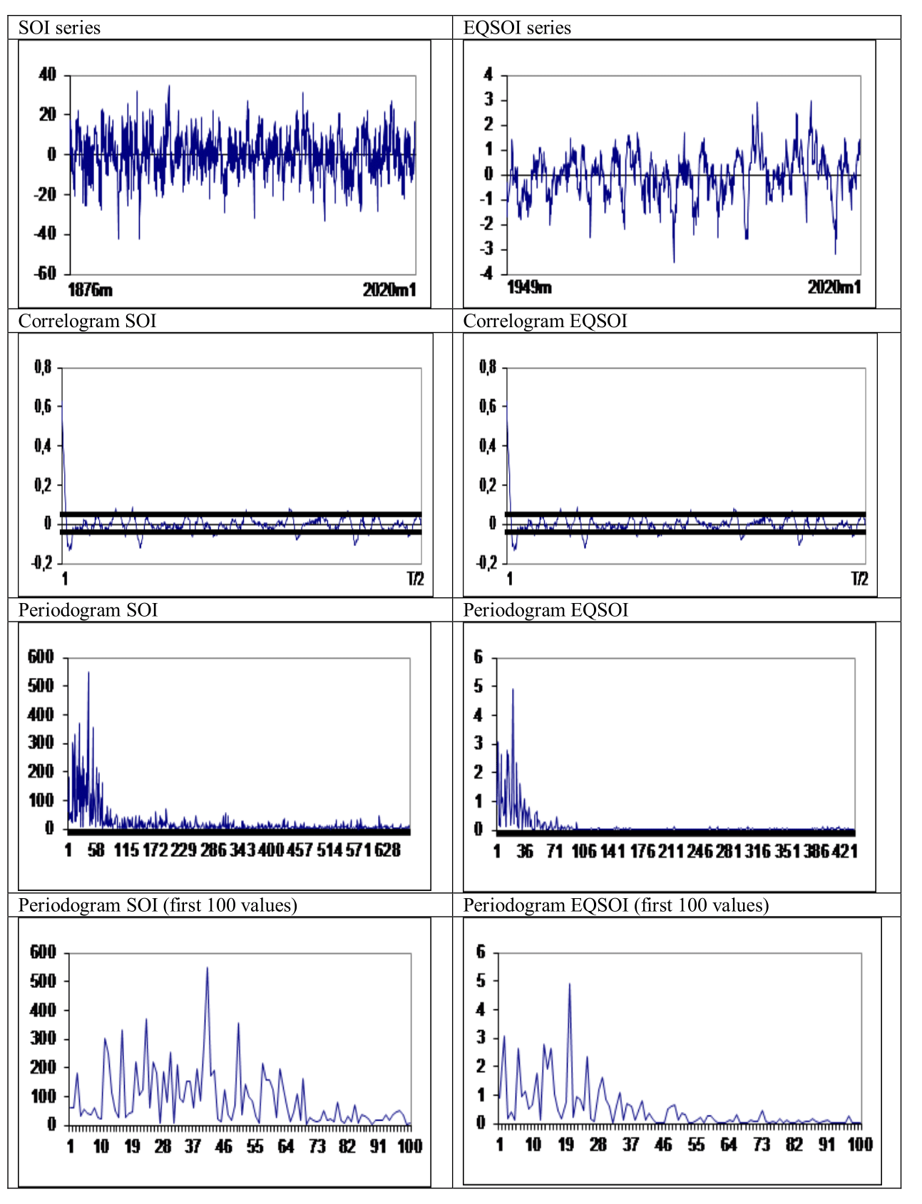
Figure 2 Time series plots, correlograms and periodograms.

It was considered the model given by Equation (5) where x_t refers to the original data (and its mean-substracted values) and u_t is described in terms of a white noise process or by employing the model of Bloomfield⁴⁶ that allows for non-parametric autocorrelation, approximating highly parameterized AR structures with very few parameters. Table 2 displays the estimates of d and their associated 95% confidence intervals

Starting with the SOI, it was observed that the estimated values of d are 0.29 and 0.28, respectively, with uncorrelated and autocorrelated (Bloomfield) errors when using the original data, and the values are slightly smaller (0.28 and 0.27) with the mean substracted data. In any case, in all cases the results support the hypothesis of long memory with the values of d in the interval (0, 0.5). Looking now at the numbers related with the cycles, it is observed that j is equal to 47 in one case (original data with uncorrelated errors) and 43 in the remaining three, corresponding to cycles of approximate length of 27 and 40 periods. Looking now at the EQSOI (in the lower part of the table) the length of the cycles is approximately the same (around 40 periods) while the order of integration is now somehow smaller, with values between 0.21 and 0.23 and thus showing a lower degree of persistence though still displaying a long memory pattern.^47–52

In this article the time series properties of the SOI and EQSOI series has been examined by using statistical techniques based on long memory, and in particular, taking into account the fact that the periodograms of the series display the highest peaks at values away from zero. Using a model based on Gegenbauer polynomials it is shown that the order of integration of the series are in the interval (0, 0.5) and thus showing a long memory mean reverting pattern, with the length of the cycles being approximately around 40 periods, which is consistent with the literature that claims that the SOI and EQSOI series have a periodicity of about 3-7 years.

It We should have been taken into account that the approach employed in this paper is simply one of the many modelling frameworks that can be used to describe these series. One advantage of our model is clearly its simplicity and its consistency with the values observed in the periodograms of the series. Note, however, that other alternatives, allowing for example non-linear deterministic trends like those based on Chebyshev polynomials in time,⁴⁹ Fourier functions⁵¹ or neural networks⁵² can also be used to describe these and other geophysical quasi-periodic data.

None.

The author declares there is no conflicts of interest.

1. Varotsos CA, Cracknell AP, Efstathiou MN. The global signature of the El Niño/La Niña Southern Oscillation. International Journal of Remote Sensing. 2018;39:5965–5977.
2. Roberts A, Guckenheimer J, Widiasih E, et al. Mixed-Mode Oscillations of El Nino–Southern Oscillation. Journal of the Atmospheric Sciences. 2016;73:1755– 1766.
3. Tudhope AW, Chilcott CP, McCulloch MT, et al. Variability in the El Niño-Southern Oscillation through a Glacial-Interglacial Cycle. Science. 2001;291(5508):1511–1517.
4. Barlow M, Nigam S, Berbery EH. ENSO, Pacific decadal variability, and US summertime precipitation, drought, and stream flow. Journal of Climate. 2001;14:2105–2128.
5. Pielke RA, Landsea CN. La Niña, El Niño and Atlantic Hurricane Damages in the United States. Bulletin of the American Meteorological Society. 1999;80:2027–2034.
6. Cane MA. El Niño in history: storming through the ages. Journal of World History. 2004;15(1):87–88.
7. Alajo SO, Nakavuma J, Erume J. Cholera in endemic districts in Uganda during El Niño rains: 2002–2003. Afr Health Sci. 2006;6(22):93–97.
8. Miyakawa T, Yashiro H, Suzuki T, et al. A madden-julian oscillation event remotely accelerates ocean upwelling to abruptly terminate the 1997/1998 super El Niño. Geophysical Research Letters. 2017;44:9489–9495.
9. Gómez-Martínez G, Pérez-Martín MA, Estrela-Monreal T, et al. North Atlantic Oscillation as a Cause of the Hydrological Changes in the Mediterranean (Júcar River, Spain). Water Resources Management. 2018;32:2717–2734.
10. Verbist K, Robertson AW, Cornelis WM, et al. Seasonal Predictability of Daily Rainfall Characteristics in Central Northern Chile for Dry-Land Management. Journal of Applied Meteorology and Climatology. 2010;49:1938–1955.
11. Meza FJ. Recent trends and ENSO influence on droughts in Northern Chile: An application of the Standardized Precipitation Evapotranspiration Index. Weather Climate Extremes. 2013;1:51–58.
12. Wang H, Kumar A. Assessing the impact of ENSO on drought in the U.S. Southwest with NCEP climate model simulations. Journal of Hydrology. 2015;526:30–41.
13. Zolotokrylin AN, Titkova TB, Brito-Castillo L. Wet and dry patterns associated with ENSO events in the Sonoran Desert from, 2000–2015. Journal of Arid Environments. 2016;134:21–32.
14. Mishra AK, Singh VP. A review of drought concepts. Journal of Hydrology. 2010;391:202– 216.
15. Arndt DS, Baringer MO, Johnson MR. State of the Climate in 2009. Bulletin of the American Meteorological Society. 2010;91(7):S1–S224.
16. Wong G, Lanen HAJ van, Torfs PJJF. Probabilistic analysis of hydrological drought characteristics using meteorological drought. Hydrological Sciences Journal. 2013;58:253–270.
17. Shiferaw B, Tesfaye K, Kassie M, et al. Managing vulnerability to drought and enhancing livelihood resilience in sub Saharan Africa: Technological, institutional and policy options. Weather and Climate Extremes. High Level Meeting on National Drought Policy. 2014;3:67–79.
18. Haile M. Weather patterns, food security and humanitarian response in sub Saharan Africa. Philosophical Transactions of the Royal Society of London. Series B, Biological Sciences. 1994;360:2169–2182.
19. Barua S, Ng AWM, Perera BJC. Drought Assessment and Forecasting: A Case Study on the Yarra River Catchment in Victoria, Australia. Australasian Journal of Water Resources. 2015;15:95–108.
20. Zambrano Mera YE, Rivadeneira Vera JF, Pérez-MartínMÁ. Linking El Niño Southern Oscillation for early drought detection in tropical climates: The Ecuadorian coast. The Science of The Total Environment. 2018;643:193–207.
21. Zheng B, Chapman S, Chenu K. The Value of Tactical Adaptation to El Niño–Southern Oscillation for East Australian Wheat. Climate. 2018;6:77.
22. Hu S, Fedorov AV. The extreme El Nino of 2015–2016: the role of westerly and easterly wind bursts and preconditioning by the failed 2014 event. Climate Dynamics. 2019;52:7339–7357.
23. Demirer R, Gupta R, Nel J, et al. Effect of rare disaster risks on crude oil: evidence from El Nino from over 140 years of data. Working Papers 2020104, University of Pretoria, Department of Economics. 2020.
24. Bouri E, Gupta R, Pierdzioch C, et al. El Niño and forecastability of oil-price realized volatility. Theoretical and Applied Climatology. 2021;144:1173–1180.
25. Demirer R, Gupta R, Suleman MT, et al. Time varying rare disaster risks, oil returns and volatility. Energy Economics. 2018;75:239–248.
26. Gil-Alana LA. Statistical model for the temperatures in the Northern hemisphere using fractional integration techniques. Journal of Climate. 2005;18(24):5537–5369.
27. Gil-Alana LA. Cyclical long‐range dependence and the warming effect in a long temperature time series. International Journal of Climatology. 2008;28(11):1435–1443.
28. Gil-Alana LA. Linear and segmented trends in sea surface temperature data. Journal of Applied Statistics. 2015;42(7):1531–1546.
29. Ercan A, Kavvas ML, Abbasov RK. Long-range dependence and sea level forecasting. Springer International Publishing. 2013;1–51.
30. Bunde A. Long-term memory in climate: Detection, extreme events and significance of trends, Chapter 11 in Nonlinear and Stochastic Climate Dynamics, edited by Christian L. E. Franzke and Terence O'Kane: Cambridge University Press. 2017.
31. Yuan N, Fu Z, Liu S. Long-term memory in climate variability: A new look based on fractional integral techniques. Journal of Geophysical Research: Atmospheres. 2013;118(12):962–969
32. Yuan N, Huang Y, Duan J, et al. On climate prediction; how much can we expect from climate memory? Climate Dynamics. 2019;52(1–2):855–864.
33. Wu H, Peiris S. An introduction to vector Gegenbauer processes with long memory, Stat (The ISI’s Journal for the Rapid Dissmination of Statistics Research). 2018;7(1):e197.
34. Barani S, Cristofaro L, Taroni M, et al. Long Memory in Earthquake Time Series: The Case Study of the Geysers Geothermal Field. Frontiers in Earth Science. 2021;9:563649.
35. Li XX, Song YF, Sivakuman BY, et al. Detection of trends types in surface air temperatures in China. Journal of Hydrology. 2021;596:126061.
36. Magnus W, Oberhettinger F, Soni RP. Formulas and Theorems for the Special Functions of Mathematical Physics. Springer, Berlin. 1966.
37. Gray H L, Yhang N, Woodward WA. On generalized fractional processes. Journal of Time Series Analysis. 1989;10:233–257.
38. Gray HL, Yhang N, Woodward WA. On generalized fractional processes. A correction. Journal of Time Series Analysis. 1994;15:561–562.
39. Ahtola J, Tiao GC. Distributions of least squares estimators of autoregressive parameters for a process with complex roots on the unit circle. Journal of Time Series Analysis. 1987a;8(1):1–14.
40. Ahtola J, Tiao GC. A note on asymptotic inference in autoregressive models with roots on the unit circle. Journal of Time Series Analysis. 1987b;8(1):15–18.
41. Bierens H. Complex unit roots and business cycles: Are they real? Econometric Theory. 2001;17:962–983.
42. Gil-Alana LA. Testing Stochastic Cycles in Macroeconomic Time Series. Journal of Time Series Analysis. 2001;22(4):411–430.
43. Phillip A, Chan J, Peiris S. On generalized bivariate student-t Gegenbauer long memory stochastic volatility models with leverage: Bayesian forecasting of cryptocurrencies with a focus on Bitcoin. Econometrics and Statistics. 2020;16:69–90.
44. Dissanayake G, Peiris S, Proietti T. Fractionally Differenced Gegenbauer Processes with Long Memory: A Review. Statistical Science. 2020;33(3):413–426.
45. Robinson PM. Efficient tests of nonstationary hypotheses, Journal of the American Statistical Association. 1994;89:1420–1437.
46. Bloomfield P. An exponential model in the spectrum of a scalar time series. Biometrika. 1973;60:217–226.
47. Behrenfeld MJ, Randerson JT, McClain CR, et al. Biospheric Primary Production during an ENSO Transition. Science. 2001;291(5513):2594–2597.
48. Bureau of Meteorology, Australian Government.
49. Cuestas FJ, Gil-Alana LA. A nonlinear approach with long range dependence based on Chebyshev polynomials in time. Studies in Nonlinear Dynamics and Econometrics. 2016;23.
50. Gil-Alana LA, Romero-Rojo F. A persistent cyclical pattern in the SOI and EQSOI series, Research Square. 2022.
51. Gil-Alana LA, Yaya OS. Testing fractional unit roots with non-linear smooth break approximations using Fourier functions. Journal of Applied Statistics. 2021;48(13-15):2542–2559.
52. Yaya OS, Ogbonna OE, Furuoka F, et al. New Unit Root Test for Unemployment Hysteresis Based on the Autoregressive Neural Network. Oxford Bulletin of Economics and Statistics. 2021;83(4):960–981.