Suitable rainfall-Intensity-Duration-Frequency (IDF) models for Uyo City were developed using the statistical method of least-squares. A total of 18 rainfall models were developed based on 10 years rainfall data. These models are categorically grouped into two sets. The first set contains 10 rainfall models which represent inverse relationship between rainfall intensities and duration for specified frequencies called Intensity-Duration-Models. The second set contains 8 rainfall models which represent rainfall intensities and frequencies for specified duration called Intensity-Frequency Model. The two sets of models developed in this research recorded high and positive values of coefficient of correlation, an indication of good curve fitting with values of Intensity-Duration Models ranging from 0.948 to 0.977 and intensity frequency model ranging from 0.641 to 0.938. These set of models developed will serve as valuable tools for predicting rainfall events in Uyo City as well as for use in the design of hydraulic structures, urban drainage and flood control.

Keywords: Rainfall modeling, Intensity, Duration, Frequency, Least squares, Uyo City

Rainfall models can be expressed mathematically to represent a relationship between Intensity, Duration & Frequency (IDF). An IDF model provides the basic probabilistic rainfall information for runoff estimation and establishes a statistical basis for design, using the return period as the measure of frequency of failure.¹⁻⁴ The IDF curves are standard tools of hydrologic risk analysis and design. Rainfall of a place can be completely defined if the intensities, durations and frequencies of the various storms occurring at that place are known. A major problem in rainfall analysis is the interpretation of past record of rainfall events in terms of future probabilities of occurrence.^5,6 Whenever an intense rain occurs, its magnitude and duration are generally known from the meteorological readings. This available data can be used to determine the frequencies of the various rains usually referred to as frequency analysis. The frequency-data for storms of various durations so obtained can be represented by Intensity-Duration-frequency Curves. Due to unavailability of rainfall data in most developing countries like Nigeria, rainfall frequency studies are very limited with only few meteorological stations usually at airport across the country. All stations where records exist, because of equipment failures continuous records for upwards of 30 years is very rare.⁵ Thus, the need for engineers to analyze available data more critically for proper planning and design of hydraulic structures is very necessary.^7,8 The aim of this study is to develop and calibrate two sets of rainfall models using observed rainfall amounts and durations. The first is the intensity- duration model of quotient formula while the second is the intensity-return period model of power law. The developed models are to find great application in design of storm-water drains, culverts, erosion protection structures, etc.

Study area: Uyo city is the state capital of Akwa Ibom, strategically located within the oil rich Niger Delta Southern of Nigeria and bounded to the South by Atlantic Ocean. It has coordinates of latitude 5⁰2’N and longitude 7⁰55’E and it is situated at elevation 45 meters above mean sea level (Figure 1).

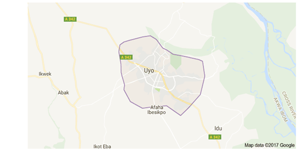
Figure 1 Map of study area, Uyo Nigeria.

Data collection: The rainfall data for Uyo City were obtained from the archives of the meteorological observatory, Department of Oceanography and Regional Planning, University of Uyo. The rainfall data obtained covered the period between 2002 and 2011.

Data analysis: Selected rainfall durations of 15, 30, 45, 60, 90, 120, 180 and 300 minutes were extracted from the rainfall data and the maximum intensities computed from Equation (1).

$i=\frac{A}{t}$ (1)

Where i: Intensity in mm/hr; A: Amount of rainfall in mm; t: Duration of rainfall in hours

The resulting intensity values evaluated from Equation (1) are ranked in decreasing order of magnitude such that the largest value is assigned 1. Return period is then computed using the Weilbull’s plotting position formula⁹ as:

$P\left(x_m\right)\text{}=\frac{m}{n+1}$ (2)

Where: $P\left(x_m\right)$ Probability of exceedence of variate x­_m­; m: Rank of descending values with largest equal to 1; n: Number of years of record

Rainfall intensities and durations are tabulated against selected frequencies of 1.1, 1.22, 1.38, 1.57, 1.83, 2.2, 2.75, 3.7, 5.5 and 11 years. Next, the inverses of intensities were obtained to establish the relationship between rainfall intensity and duration for specified frequency.

Intensity-duration quotient models: Frequencies of rainfall events calculated as the reciprocal of their corresponding probabilities are as presented in Table 1. Many formulas have been proposed in the past to fit rainfall-Intensity-Duration-Frequency Curves, but most of them are in a form with intensity inversely proportional to duration.^5‒10 The quotient model was used for the development of relationship between intensity of rainfall and its duration at specific return period. The quotient model is given by⁹ as;

$i=\frac{a}{t+b}$ (3)

Where i: rainfall intensity (mm/hr); t: rainfall duration (hr); a, b: regional constants

Equation (3) is linearized by taking its reciprocal to become Equation (4):

$y=a_0+a_{1}x$ (4)

Where: $y=1/i;$

$a_0=b/a;a_1=1/a.$

Equation (4) was solved using regression analysis via XLSTAT to produce the intensity duration models shown in Table 2. The rainfall intensity duration curves are shown in Figure 2. Apparently, the quotient model was calibrated by using the rainfall data on intensities and durations (Table 1) to obtain the regional constants of and in Equation (3) as presented in Table 3.

Intensity-return period power models: The power model was employed in developing relationship between rainfall intensity and return period at specified duration. The power model⁵ is given by:

$i=a{R}^b$ (5)

Where I, rainfall intensity (mm/hr); R, return period (years); &, regional constants

Equation (5) is linearized by logarithmic approach, viz;

$\log i=\log a+b\log R$ (6)

Where: $a_1=band{a}_0=\log a$

Regression analysis was equally employed to solve and calibrate Equation (6) using data from (Table 1) to produce the rainfall intensity-frequency models shown in Table 2. The Intensity Frequency Curves are shown in Figure 3.

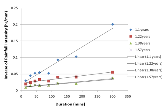
Figure 2 Inverse of Rainfall Intensity duration curves for specified frequencies for Uyo City.

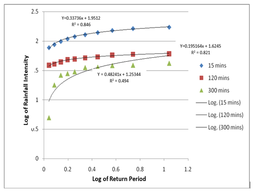
Figure 3 Rainfall Intensity return period power model for specified durations, option -1.

The first set of rainfall models involved finding solution of the quotient formula of Equation (3) using available rainfall intensity duration data for specified frequencies of 1.1-11 years. A total of 10 rainfall models were developed as presented in Table 3 with high and positive values of coefficient of correlations of 0.948 to 0.977. The second set of rainfall models involved finding solution of the power model of Equation (5) using rainfall intensities frequency data for specified durations of 15-300 minutes. A total of 8 models were obtained as presented in Table 2 with moderate to high positive values of coefficients of correlation of 0.641 to 0.938 indicating good curve fittings. The plots of intensities against duration for the specified frequencies in Figure 2 and intensities against frequencies for the specified durations in Figure 3 formed a good basis for the predicted results. On the basis of these plots, Uyo city rainfall pattern can be characterized by the following observations. a. The curves are parallel; they do not cross each other; b. High and positive values of coefficients of correlation indicate best curve fittings; c. Higher return periods correspond with higher rainfall intensities for a given duration.¹¹

Based on the results of this study the following conclusion can be drawn:

1. The IDF models for Uyo City and their graphical equivalents have been developed from extracted rainfall data subjected to regression analyses which gave high and positive coefficient of correlation values as indication of good curve fitting.
2. The IDF models as derived are similar to those encountered in Engineering practice which will serve as valuable and reliable tools for engineers and hydrologists for predicting rainfall events as well as basic rainfall information for design of drains in Uyo City.

None.

None.

1. Nwaogazie IL, Ologhadien I. Rainfall Intensity-Duration-Frequency Models for Selected Cities in Southern Nigeria. Standard Scientific Research and Essays. 2014;2(10):509−515.
2. Abubakari S. Development of Intensity-Duration-Frequency Curves for Kumasi. MSc Thesis: Kwame Nkrumah University of Science and Technology, Ghana; 2013. p. 1‒112.
3. Akpan SU, Okoro BC. Developing Rainfall Intensity-Duration-Frequency Models for Calabar City, South-South, Nigeria. American Journal of Engineering Research. 2013;2(6):19−24.
4. Nwadike CN. Developing Rainfall Models for Enugu City. MEng Thesis, Dept of Civil Engineering, Imo, Nigeria: Federal University of Technology, Owerri (FUTO); 2008.
5. Nwaogazie IL, Duru EO. Developing Rainfall-Intensity-Duration-Frequency Models for Port Harcourt City. NSE Technical Transaction. 2002;37(2):19‒32.
6. Udo Inyang CU, Edem DI. Analysis of Rainfall Trends in Akwa Ibom State, Nigeria. Journal of Environment and Earth Science. 2012;2(8):1−12.
7. FMW H. Federal Republic of Nigeria Highway Design Manual (Part-1), Federal Ministry of Works; 2006.
8. Okonkwo GI, Mbajiorgu CC. Rainfall Intensity-Duration-Frequency Analysis for Southeastern Nigeria. Agric Eng Int: The CIGR journal. 2010;12(1):22‒30.
9. Nwaogazie IL. Probability and Statistics for Science and Engineering Practice. Enugu, Nigeria: De- Adroit Innovation; 2011. p. 1−288.
10. Nwaogazie Ify L, Okonkwo S, Chukwuemeka. Rainfall-Intensity-Duration-Frequency Modeling and Comparative Analysis of Developed Models for Abakaliki, Ebonyi State, Nigeria. International Journal of Trend in Research and Development. 2017;4(2):776‒783.
11. Nwoke UH. Rainfall Intensity-Frequency Regime for Owerri South-East Nigeria. Continental J. Environmental Sciences. 2013;7(1): 1−7.