Submit manuscript...
eISSN: 2577-8242

Fluid Mechanics Research International Journal

Research Article Volume 2 Issue 5

Turbulence modeling of drag reducing fluid flow using modified k-ω model

Lotfy Rabie H, Mohamed Fouda S, Mohamed Awad M

Department of Mechanical Power Engineering, Mansoura University, Egypt

Correspondence: Lotfy Hassan Rabie, Department of Mechanical Power Engineering, Faculty of Engineering, Mansoura University, El-Mansoura, Egypt

Received: December 23, 2017 | Published: November 27, 2018

Citation: Rabie HL, Fouda SM, Awad MM. Turbulence modeling of drag reducing fluid flow using modified k- ? model. Fluid Mech Res Int J. 2018;2(5):219-228. DOI: 10.15406/fmrij.2018.02.00041

Download PDF

Abstract

In the present study, a standard eddy viscosity turbulence model for Newtonian fluids has been developed to predict the drag reduction and the mean velocity profile of drag reducing fluids. In addition, this model is an extension of FENE-P eddy viscosity model for viscoelastic fluids without using any additional constitutive equation. In this work, the first section is concerned with developing a new correlation for the eddy viscosity equation, which depends on the flow and rheological parameters, based on the Direct Numerical Simulation (DNS) data. For this purpose, a User Defined Function (UDF) was interpreted to Fluent 16.1 solver to supersede the Newtonian eddy viscosity with a new average eddy viscosity which is pertinent to the characteristics of the polymer solution. In the second section, the validity of the created model was compared with the results of experiments and DNS model for fully developed turbulent channel flow for other investigators.

The developed model predictions for the drag reduction and the mean velocity profile showed good agreement with the DNS model and experimental results at low and intermediate drag reduction regions (i.e. ). In contrast, in high drag reduction and near Virk’s asymptote region (i.e. ), the accuracy of the model was lost. Finally, the present model is an extension of Reynolds averaged Navier Stokes equation based on standard model. Consequently, the model can be more practical at higher values of Reynolds number and complex geometries other than the DNS model, which poses benefits only at lower values of Reynolds number and simple geometry.

Introduction

The addition of a few weight parts per million (wppm) of long-chain flexible polymer molecules to the turbulent flow of a solvent can drastically improve the heat transfer and reduce the turbulent friction. This process is also known as a drag reduction. Always, higher molecular weight polymers give better drag reduction performance. However, the addition of a minute amount of polymer in the working fluid reduces the turbulent eddies due to suppressing the formation and propagation turbulent bursts in the buffer layer region. Consequently, resulting in losses reduction in hydraulic energy due to a chaotic and random motion.1 This phenomenon was initially discovered by.2 Since then drag reduction by polymer additives subsequently undergoes extensive researches due to continuous increase in its practical applications, such as, long distance fluid transportation and in cooling and heating systems. Therefore, developing the numerical models becomes a vital issue to solve these types of practical engineering problems. To understand the polymer behavior and why drag reduction occur, many experimental and numerical studies had been carried out in the fields of chemistry and fluid mechanics. The exact mechanism of drag reduction for polymer solutions is still vague due to the complexity of flow.

There are two phenomena in drag reducing fluid flow as following:

  1. Onset of drag reduction.
  2. Maximum Drag Reduction (MDR).

The onset of drag reduction is the criteria which must be met before a given polymer solution can display any drag reducing effects in turbulent flow. The onset of drag reduction relies on polymer solution parameters and Reynolds number. If these criteria are not met, the flow behaves similar to a Newtonian fluid and the drag reduction is not occurred. The mean velocity profile of Newtonian fluids can be expressed by:

u + = y +                    y + <11.6  MathType@MTEF@5@5@+= feaagKart1ev2aaatCvAUfeBSjuyZL2yd9gzLbvyNv2CaerbuLwBLn hiov2DGi1BTfMBaeXatLxBI9gBaerbd9wDYLwzYbItLDharqqtubsr 4rNCHbGeaGqiVu0Je9sqqrpepC0xbbL8F4rqqrFfpeea0xe9Lq=Jc9 vqaqpepm0xbba9pwe9Q8fs0=yqaqpepae9pg0FirpepeKkFr0xfr=x fr=xb9adbaqaaeGaciGaaiaabeqaamaabaabaaGcbaqcLbsaqaaaaa aaaaWdbiaadwhajuaGpaWaaWbaaSqabeaajugWa8qacqGHRaWkaaqc LbsacqGH9aqpcaWG5bqcfa4damaaCaaaleqabaqcLbmapeGaey4kaS caaKqzGeGaaiiOaiaacckacaGGGcGaaiiOaiaacckacaGGGcGaaiiO aiaacckacaGGGcGaaiiOaiaacckacaGGGcGaaiiOaiaacckacaGGGc GaaiiOaiaacckacaGGGcGaamyEaSWdamaaCaaabeqaaKqzadWdbiab gUcaRaaajugibiabgYda8iaaigdacaaIXaGaaiOlaiaaiAdakiaacc kaaaa@5E20@ (sub layer region) (1)

u + =2.5ln y + +5.5          y + 11.6  MathType@MTEF@5@5@+= feaagKart1ev2aaatCvAUfeBSjuyZL2yd9gzLbvyNv2CaerbuLwBLn hiov2DGi1BTfMBaeXatLxBI9gBaerbd9wDYLwzYbItLDharqqtubsr 4rNCHbGeaGqiVu0Je9sqqrpepC0xbbL8F4rqqrFfpeea0xe9Lq=Jc9 vqaqpepm0xbba9pwe9Q8fs0=yqaqpepae9pg0FirpepeKkFr0xfr=x fr=xb9adbaqaaeGaciGaaiaabeqaamaabaabaaGcbaqcLbsaqaaaaa aaaaWdbiaadwhal8aadaahaaqabeaajugWa8qacqGHRaWkaaqcLbsa cqGH9aqpcaaIYaGaaiOlaiaaiwdaciGGSbGaaiOBaiaadMhal8aada ahaaqabeaajugWa8qacqGHRaWkaaqcLbsacqGHRaWkcaaI1aGaaiOl aiaaiwdacaGGGcGaaiiOaiaacckacaGGGcGaaiiOaiaacckacaGGGc GaaiiOaiaacckacaWG5bqcfa4damaaCaaaleqabaqcLbmapeGaey4k aScaaKqzGeGaeyyzImRaaGymaiaaigdacaGGUaGaaGOnaOGaaiiOaa aa@5B33@ (buffer layer region) (2)

Where  is the normalized velocity i.e., , u is the local velocity and  is the frictional velocity, is the normalized distance from a wall i.e., , v is the kinematic viscosity and y is the normal distance from a wall. When the drag reduction value increases,3 observed that, the log law is shifted by  in buffer layer region and the slope of line is not changed. It was concluded that, the mean velocity profile in buffer layer can be written in the form of:

u + =2.5ln y + +5.5+ S + MathType@MTEF@5@5@+= feaagKart1ev2aaatCvAUfeBSjuyZL2yd9gzLbvyNv2CaerbuLwBLn hiov2DGi1BTfMBaeXatLxBI9gBaerbd9wDYLwzYbItLDharqqtubsr 4rNCHbGeaGqiVu0Je9sqqrpepC0xbbL8F4rqqrFfpeea0xe9Lq=Jc9 vqaqpepm0xbba9pwe9Q8fs0=yqaqpepae9pg0FirpepeKkFr0xfr=x fr=xb9adbaqaaeGaciGaaiaabeqaamaabaabaaGcbaqcLbsaqaaaaa aaaaWdbiaadwhajuaGpaWaaWbaaSqabeaajugWa8qacqGHRaWkaaqc LbsacqGH9aqpcaaIYaGaaiOlaiaaiwdaciGGSbGaaiOBaiaadMhaju aGpaWaaWbaaSqabeaajugWa8qacqGHRaWkaaqcLbsacqGHRaWkcaaI 1aGaaiOlaiaaiwdacqGHRaWkcaqGtbqcfa4damaaCaaaleqabaqcLb mapeGaey4kaScaaaaa@4C5A@ (3)

In addition,3 found a universal asymptote which is not related to both of the type and the polymer concentration in the solution. This phenomenon is known as maximum drag reduction (MDR). Based on experimental data,3 proposed the mean velocity profile in buffer layer region at (MDR) by:

u + =11.7ln y + 17 MathType@MTEF@5@5@+= feaagKart1ev2aaatCvAUfeBSjuyZL2yd9gzLbvyNv2CaerbuLwBLn hiov2DGi1BTfMBaeXatLxBI9gBaerbd9wDYLwzYbItLDharqqtubsr 4rNCHbGeaGqiVu0Je9sqqrpepC0xbbL8F4rqqrFfpeea0xe9Lq=Jc9 vqaqpepm0xbba9pwe9Q8fs0=yqaqpepae9pg0FirpepeKkFr0xfr=x fr=xb9adbaqaaeGaciGaaiaabeqaamaabaabaaGcbaqcLbsaqaaaaa aaaaWdbiaadwhal8aadaahaaqabeaajugWa8qacqGHRaWkaaqcLbsa cqGH9aqpcaaIXaGaaGymaiaac6cacaaI3aGaciiBaiaac6gacaWG5b WcpaWaaWbaaeqabaqcLbmapeGaey4kaScaaKqzGeGaeyOeI0IaaGym aiaaiEdaaaa@46AF@ (4)                                                                                                                

There are three regions of drag reduction as the following:

  1. Low region (DR<30 %) MathType@MTEF@5@5@+= feaagKart1ev2aaatCvAUfeBSjuyZL2yd9gzLbvyNv2CaerbuLwBLn hiov2DGi1BTfMBaeXatLxBI9gBaerbd9wDYLwzYbItLDharqqtubsr 4rNCHbGeaGqiVu0Je9sqqrpepC0xbbL8F4rqqrFfpeea0xe9Lq=Jc9 vqaqpepm0xbba9pwe9Q8fs0=yqaqpepae9pg0FirpepeKkFr0xfr=x fr=xb9adbaqaaeGaciGaaiaabeqaamaabaabaaGcbaqcLbsaqaaaaa aaaaWdbiaacIcacaWGebGaamOuaiabgYda8iaaiodacaaIWaGaaiiO aiaacwcacaGGPaaaaa@3DE6@
  2. Intermediate region (30 %DR50 %) MathType@MTEF@5@5@+= feaagKart1ev2aaatCvAUfeBSjuyZL2yd9gzLbvyNv2CaerbuLwBLn hiov2DGi1BTfMBaeXatLxBI9gBaerbd9wDYLwzYbItLDharqqtubsr 4rNCHbGeaGqiVu0Je9sqqrpepC0xbbL8F4rqqrFfpeea0xe9Lq=Jc9 vqaqpepm0xbba9pwe9Q8fs0=yqaqpepae9pg0FirpepeKkFr0xfr=x fr=xb9adbaqaaeGaciGaaiaabeqaamaabaabaaGcbaqcLbsaqaaaaa aaaaWdbiaacIcacaaIZaGaaGimaiaacckacaGGLaGaeyizImQaamir aiaadkfacqGHKjYOcaaI1aGaaGimaiaacckacaGGLaGaaiykaaaa@4392@
  3. Maximum region (DR>50 %) MathType@MTEF@5@5@+= feaagKart1ev2aaatCvAUfeBSjuyZL2yd9gzLbvyNv2CaerbuLwBLn hiov2DGi1BTfMBaeXatLxBI9gBaerbd9wDYLwzYbItLDharqqtubsr 4rNCHbGeaGqiVu0Je9sqqrpepC0xbbL8F4rqqrFfpeea0xe9Lq=Jc9 vqaqpepm0xbba9pwe9Q8fs0=yqaqpepae9pg0FirpepeKkFr0xfr=x fr=xb9adbaqaaeGaciGaaiaabeqaamaabaabaaGcbaqcLbsaqaaaaa aaaaWdbiaacIcacaWGebGaamOuaiabg6da+iaaiwdacaaIWaGaaiiO aiaacwcacaGGPaaaaa@3DEC@

Interest in developing turbulence models for the prediction of drag reducing fluids flow has grown over recent years. The main object of drag reducing fluids researches is to develop a viscoelastic turbulence model which is able to predict correctly the drag reduction value and the mean velocity profile in all drag reduction regions and for any polymer solution. The first turbulence models for viscoelastic fluids flow originated at 1970’s by4 and.5 The limited range illustrates how complexity, difficulty and weakly of such models, since they depend on large number of parameters that have different values for each polymer solution in each flow situation. Also these earlier models had no obvious link to the polymer rheology. More physically-based models for purely viscous fluids of variable viscosity were investigated by.6 Based on the same concept, Pinho and co-workers,7-9 later adopted a generalized Newtonian fluid constitutive equation by introducing some extensional viscosity influences that include the deformation tensor rate. These models tried to describe the polymer rheology by purely viscous constitutive equation such as the power law model for yield stress fluids. However, these models are not based on a true viscoelastic constitutive and it was unable to capture all features of elastic fluids.

It is well known that, the DNS constitutive models, which describe the dilute polymer solutions rheology well like FENE-P model, were adopted for the turbulence closures development. The FENE-P is the more accurate model for these complex flow situations, regardless that there are still some discrepancies between the measured intensities of drag reduction and calculated (by DNS) specially at higher drag reduction region.10 Therefore,11-13used extensively the FENE-P model, which is coupled with DNS model, to simulate the rheology of the fluids in turbulent flows. However, little number of publications based on Giesekus model14 and Oldroyd-B model,15 which are suitable for the surfactant flow, were coupled with DNS model to simulate the FENE-P fluids. In some cases, the DNS data was processed to provide Reynolds average data16,17 and explain the vortex dynamics.18,19 Though, there is an absence of detailed experimental evaluation, DNS simulation can provide a validating guidelines for both Reynolds Averaged Navier-Stokes (RANS) equations and Large eddy simulations (LES) at relatively low Reynolds number and simple geometry such as a flat plate flow or a fully developed channel flow. On contrary, at high Reynolds number and complex geometry such as flow past ships, the DNS simulation are impractical, because the number of degree of freedom for DNS R e 9/4 MathType@MTEF@5@5@+= feaagKart1ev2aaatCvAUfeBSjuyZL2yd9gzLbvyNv2CaerbuLwBLn hiov2DGi1BTfMBaeXatLxBI9gBaerbd9wDYLwzYbItLDharqqtubsr 4rNCHbGeaGqiVu0Je9sqqrpepC0xbbL8F4rqqrFfpeea0xe9Lq=Jc9 vqaqpepm0xbba9pwe9Q8fs0=yqaqpepae9pg0FirpepeKkFr0xfr=x fr=xb9adbaqaaeGaciGaaiaabeqaamaabaabaaGcbaqcLbsaqaaaaa aaaaWdbiabg2Hi1kaadkfacaWGLbWcdaahaaqcfayabeaajugWaiaa iMdacaGGVaGaaGinaaaaaaa@3E03@ .

Consequently, the need to develop turbulence models based on RANS equations by using FENE-P model has been appeared in recent years.13developed a Reynolds average kind of turbulence model based on FENE-P models. The mathematical expressions for eddy viscosity of RANS mixing length model in three regions of drag reduction was presented based on the DNS results of the FENE-P model. Then 20 proposed a model that is considered as an extension of the low Reynolds number kε MathType@MTEF@5@5@+= feaagKart1ev2aaatCvAUfeBSjuyZL2yd9gzLbvyNv2CaerbuLwBLn hiov2DGi1BTfMBaeXatLxBI9gBaerbd9wDYLwzYbItLDharqqtubsr 4rNCHbGeaGqiVu0Je9sqqrpepC0xbbL8F4rqqrFfpeea0xe9Lq=Jc9 vqaqpepm0xbba9pwe9Q8fs0=yqaqpepae9pg0FirpepeKkFr0xfr=x fr=xb9adbaqaaeGaciGaaiaabeqaamaabaabaaGcbaqcLbsaqaaaaa aaaaWdbiaadUgacqGHsislcqaH1oqzaaa@3A29@ model of Nagano Y et al.21 for Newtonian fluids.20 used a two additional constitutive equation based on FENE-P model and developed closures of terms in conformation tensor equation based on the results of Housiadas KD et al.18 These earlier models were typically correlated and developed based on the DNS data and were only used to understand and predict the low and intermediate drag reduction regions.22 developed a kε MathType@MTEF@5@5@+= feaagKart1ev2aaatCvAUfeBSjuyZL2yd9gzLbvyNv2CaerbuLwBLn hiov2DGi1BTfMBaeXatLxBI9gBaerbd9wDYLwzYbItLDharqqtubsr 4rNCHbGeaGqiVu0Je9sqqrpepC0xbbL8F4rqqrFfpeea0xe9Lq=Jc9 vqaqpepm0xbba9pwe9Q8fs0=yqaqpepae9pg0FirpepeKkFr0xfr=x fr=xb9adbaqaaeGaciGaaiaabeqaamaabaabaaGcbaqcLbsaqaaaaa aaaaWdbiaadUgacqGHsislcqaH1oqzaaa@3A29@ model based on the v 2 f MathType@MTEF@5@5@+= feaagKart1ev2aaatCvAUfeBSjuyZL2yd9gzLbvyNv2CaerbuLwBLn hiov2DGi1BTfMBaeXatLxBI9gBaerbd9wDYLwzYbItLDharqqtubsr 4rNCHbGeaGqiVu0Je9sqqrpepC0xbbL8F4rqqrFfpeea0xe9Lq=Jc9 vqaqpepm0xbba9pwe9Q8fs0=yqaqpepae9pg0FirpepeKkFr0xfr=x fr=xb9adbaqaaeGaciGaaiaabeqaamaabaabaaGcbaqcLbsaqaaaaa aaaaWdbiaadAhajuaGdaahaaqabeaajugWaiaaikdaaaqcLbsacqGH sislcaWGMbaaaa@3CA1@ model which is an extension of Durbin P 23 model. The Reynolds averaged polymer stress was modeled without solving the evolution equation for the polymer conformation tensor. The results showed a good agreement with DNS data while model is still limited to low and intermediate drag reduction regions. More recently,24 improved significantly the turbulence model of Pinho FT et al20 by extending its closures of terms in conformation tensor equation to the high drag reduction region and improving its general performance. For Newtonian fluids, it is known that there are problems in the kε MathType@MTEF@5@5@+= feaagKart1ev2aaatCvAUfeBSjuyZL2yd9gzLbvyNv2CaerbuLwBLn hiov2DGi1BTfMBaeXatLxBI9gBaerbd9wDYLwzYbItLDharqqtubsr 4rNCHbGeaGqiVu0Je9sqqrpepC0xbbL8F4rqqrFfpeea0xe9Lq=Jc9 vqaqpepm0xbba9pwe9Q8fs0=yqaqpepae9pg0FirpepeKkFr0xfr=x fr=xb9adbaqaaeGaciGaaiaabeqaamaabaabaaGcbaqcLbsaqaaaaa aaaaWdbiaadUgacqGHsislcqaH1oqzaaa@3A29@ turbulence models either because of the lack of natural boundary condition of, ε MathType@MTEF@5@5@+= feaagKart1ev2aaatCvAUfeBSjuyZL2yd9gzLbvyNv2CaerbuLwBLn hiov2DGi1BTfMBaeXatLxBI9gBaerbd9wDYLwzYbItLDharqqtubsr 4rNCHbGeaGqiVu0Je9sqqrpepC0xbbL8F4rqqrFfpeea0xe9Lq=Jc9 vqaqpepm0xbba9pwe9Q8fs0=yqaqpepae9pg0FirpepeKkFr0xfr=x fr=xb9adbaqaaeGaciGaaiaabeqaamaabaabaaGcbaqcLbsaqaaaaa aaaaWdbiabew7aLbaa@384C@ , and the appearance of higher-order correlations in the balance of the dissipation rate at the wall. As a result, forcing the usage of higher-order derivatives of the turbulent kinetic energy that leads to a not asymptotic behavior and consequently to numerical stiffness. So researchers tried to find an alternative to ε MathType@MTEF@5@5@+= feaagKart1ev2aaatCvAUfeBSjuyZL2yd9gzLbvyNv2CaerbuLwBLn hiov2DGi1BTfMBaeXatLxBI9gBaerbd9wDYLwzYbItLDharqqtubsr 4rNCHbGeaGqiVu0Je9sqqrpepC0xbbL8F4rqqrFfpeea0xe9Lq=Jc9 vqaqpepm0xbba9pwe9Q8fs0=yqaqpepae9pg0FirpepeKkFr0xfr=x fr=xb9adbaqaaeGaciGaaiaabeqaamaabaabaaGcbaqcLbsaqaaaaa aaaaWdbiabew7aLbaa@384C@ . Wilcox developed the kω  MathType@MTEF@5@5@+= feaagKart1ev2aaatCvAUfeBSjuyZL2yd9gzLbvyNv2CaerbuLwBLn hiov2DGi1BTfMBaeXatLxBI9gBaerbd9wDYLwzYbItLDharqqtubsr 4rNCHbGeaGqiVu0Je9sqqrpepC0xbbL8F4rqqrFfpeea0xe9Lq=Jc9 vqaqpepm0xbba9pwe9Q8fs0=yqaqpepae9pg0FirpepeKkFr0xfr=x fr=xb9adbaqaaeGaciGaaiaabeqaamaabaabaaGcbaqcLbsaqaaaaa aaaaWdbiaadUgacqGHsislcqaHjpWDkiaacckaaaa@3B7D@ model where the exact viscous terms next to the wall do not require modeling. Thus leading to better predictions without using the damping functions typical of kε MathType@MTEF@5@5@+= feaagKart1ev2aaatCvAUfeBSjuyZL2yd9gzLbvyNv2CaerbuLwBLn hiov2DGi1BTfMBaeXatLxBI9gBaerbd9wDYLwzYbItLDharqqtubsr 4rNCHbGeaGqiVu0Je9sqqrpepC0xbbL8F4rqqrFfpeea0xe9Lq=Jc9 vqaqpepm0xbba9pwe9Q8fs0=yqaqpepae9pg0FirpepeKkFr0xfr=x fr=xb9adbaqaaeGaciGaaiaabeqaamaabaabaaGcbaqcLbsaqaaaaa aaaaWdbiaadUgacqGHsislcqaH1oqzaaa@3A29@ closures.

Consequently,25 developed an eddy viscosity model based on26 kε MathType@MTEF@5@5@+= feaagKart1ev2aaatCvAUfeBSjuyZL2yd9gzLbvyNv2CaerbuLwBLn hiov2DGi1BTfMBaeXatLxBI9gBaerbd9wDYLwzYbItLDharqqtubsr 4rNCHbGeaGqiVu0Je9sqqrpepC0xbbL8F4rqqrFfpeea0xe9Lq=Jc9 vqaqpepm0xbba9pwe9Q8fs0=yqaqpepae9pg0FirpepeKkFr0xfr=x fr=xb9adbaqaaeGaciGaaiaabeqaamaabaabaaGcbaqcLbsaqaaaaa aaaaWdbiaadUgacqGHsislcqaH1oqzaaa@3A29@ model for drag reducing fluid flow. The new eddy viscosity model based on polymer rheology is an extension of Pinho FT et al20 and two additional constitutive equation were adopted. These models are typically used for drag reduction up to 50 % in low and intermediate region. Another approach to turbulence modeling was proposed by27 which is an extension of Iaccarino G et al22 but it is valid for the three regions of the drag reduction. The additional constitutive equation based on FENE-P model is not used in this model and it’s replaced with two transport equations for v2 and f. This model was modified by28 to predict the mean temperature profile and heat transfer rates in viscoelastic fluid by adding the additional terms to the energy equation. Moreover,29 modified the model developed by27 (kε  ν 2 f  model) MathType@MTEF@5@5@+= feaagKart1ev2aaatCvAUfeBSjuyZL2yd9gzLbvyNv2CaerbuLwBLn hiov2DGi1BTfMBaeXatLxBI9gBaerbd9wDYLwzYbItLDharqqtubsr 4rNCHbGeaGqiVu0Je9sqqrpepC0xbbL8F4rqqrFfpeea0xe9Lq=Jc9 vqaqpepm0xbba9pwe9Q8fs0=yqaqpepae9pg0FirpepeKkFr0xfr=x fr=xb9adbaqaaeGaciGaaiaabeqaamaabaabaaGcbaqcLbsaqaaaaa aaaaWdbiaacIcacaWGRbGaeyOeI0IaeqyTduMaeyOeI0IaaiiOaiab e27aULqbaoaaCaaabeqaaKqzadGaaGOmaaaajugibiabgkHiTiaadA gakiaacckacaGGGcGaciyBaiaac+gacaGGKbGaamyzaiaadYgacaGG Paaaaa@4B47@ to predict the velocity profiles, shear stress profiles and the percentage of friction drag reduction at high concentration solutions. The accuracy of model was lost at both of high Reynolds number and high concentration.

Based on the previous review of literature, it has been concluded that:

  1. The DNS constitutive models (like FENE-P model), which describe well the polymer rheology, are more accurate model for the turbulent drag reducing fluid flow at low values of Reynolds number and simple geometries.
  2. At higher Reynolds number values and complex geometries, the RANS models are more practical than the DNS model.
  3. For wall bounded turbulent flow, better predictions were given by the RANS kω MathType@MTEF@5@5@+= feaagKart1ev2aaatCvAUfeBSjuyZL2yd9gzLbvyNv2CaerbuLwBLn hiov2DGi1BTfMBaeXatLxBI9gBaerbd9wDYLwzYbItLDharqqtubsr 4rNCHbGeaGqiVu0Je9sqqrpepC0xbbL8F4rqqrFfpeea0xe9Lq=Jc9 vqaqpepm0xbba9pwe9Q8fs0=yqaqpepae9pg0FirpepeKkFr0xfr=x fr=xb9adbaqaaeGaciGaaiaabeqaamaabaabaaGcbaqcLbsaqaaaaa aaaaWdbiaadUgacqGHsislcqaHjpWDaaa@3A4F@ turbulence model without using additional damping function as in the case of using kε MathType@MTEF@5@5@+= feaagKart1ev2aaatCvAUfeBSjuyZL2yd9gzLbvyNv2CaerbuLwBLn hiov2DGi1BTfMBaeXatLxBI9gBaerbd9wDYLwzYbItLDharqqtubsr 4rNCHbGeaGqiVu0Je9sqqrpepC0xbbL8F4rqqrFfpeea0xe9Lq=Jc9 vqaqpepm0xbba9pwe9Q8fs0=yqaqpepae9pg0FirpepeKkFr0xfr=x fr=xb9adbaqaaeGaciGaaiaabeqaamaabaabaaGcbaqcLbsaqaaaaa aaaaWdbiaadUgacqGHsislcqaH1oqzaaa@3A29@ model
  4. Using additional FENE-P constitutive equations in RANS kω model increase the running time and simulation cost, especially at higher values of Reynolds number and complex geometries.

Hence, the objective of the present study is to investigate a new RANS kω turbulence model for drag reducing flow without using additional constitutive equations. The investigated model is based on the standard RANS kω turbulence model developed by26 and eddy viscosity model proposed by.25 A user defined function (UDF) code is interpreted to ANSYS -Fluent 16.1 solver to replace the Newtonian eddy viscosity with a new average eddy viscosity, which takes into account the flow characteristics and the polymer parameters. The predicted model will be valid for both low and intermediate drag reduction regions (DR60) , because of the limiting assumption of Resende model. The model also will be verified using DNS data for fully-developed channel flow provided by Li C et al13 and the experimental Results of Warholic M et al.30

Numerical model

Governing equations

The turbulence model developed here is based on the continuity and the Reynolds Averaged Navier Stokes (RANS) equations.

Incompressible continuity and momentum equations

The equations are written in the indicial notation of Einstein with Kronecker de (δij=1 if i=j and δij=0 if ij) . The time-averaged continuity and momentum equations for an incompressible FENE-P fluid are:

Uixi=0 (5)

ρ U i t +ρ U k U i x k = P x i + μ s 2 U i x k x k x k ( ρ u i u k ¯ )+ τ ¯ ik,p x k MathType@MTEF@5@5@+= feaagKart1ev2aaatCvAUfeBSjuyZL2yd9gzLbvyNv2CaerbuLwBLn hiov2DGi1BTfMBaeXatLxBI9gBaerbd9wDYLwzYbItLDharqqtubsr 4rNCHbGeaGqiVu0Je9sqqrpepC0xbbL8F4rqqrFfpeea0xe9Lq=Jc9 vqaqpepm0xbba9pwe9Q8fs0=yqaqpepae9pg0FirpepeKkFr0xfr=x fr=xb9adbaqaaeGaciGaaiaabeqaamaabaabaaGcbaqcLbsaqaaaaa aaaaWdbiabeg8aYLqbaoaalaaajyaGpaqaaKqzGeWdbiabgkGi2kaa dwfalmaaBaaajuaGbaqcLbmacaWGPbaajuaGbeaaaKGba+aabaqcLb sapeGaeyOaIyRaamiDaaaacqGHRaWkcqaHbpGCcaWGvbqcfa4damaa BaaajyaGbaqcLbsapeGaam4Aaaqcga4daeqaaKqba+qadaWcaaqcga 4daeaajugib8qacqGHciITcaWGvbWcdaWgaaqcfayaaKqzadGaamyA aaqcfayabaaajyaGpaqaaKqzGeWdbiabgkGi2kaadIhalmaaBaaaju aGbaqcLbmacaWGRbaajuaGbeaaaaqcLbsacqGH9aqpcqGHsisljuaG daWcaaqcga4daeaajugib8qacqGHciITcaWGqbaajyaGpaqaaKqzGe WdbiabgkGi2kaadIhalmaaBaaajuaGbaqcLbmacaWGPbaajuaGbeaa aaqcLbsacqGHRaWkcqaH8oqBjuaGpaWaaSbaaKGbagaajugib8qaca WGZbaajyaGpaqabaqcfa4dbmaalaaajyaGpaqaaKqzGeWdbiabgkGi 2Mqba+aadaahaaqcgayabeaajugWa8qacaaIYaaaaKqzGeGaamyvaS WaaSbaaKqbagaajugWaiaadMgaaKqbagqaaaqcga4daeaajugib8qa cqGHciITcaWG4bqcfa4aaSbaaeaajugWaiaadUgaaKqbagqaaKqzGe GaeyOaIyRaamiEaKqbaoaaBaaabaqcLbmacaWGRbaajuaGbeaaaaqc LbsacqGHsisljuaGdaWcaaqcga4daeaajugib8qacqGHciITaKGba+ aabaqcLbsapeGaeyOaIyRaamiEaSWaaSbaaKqbagaajugWaiaadUga aKqbagqaaaaadaqadaqcga4daeaajugibiabeg8aYLqbaoaanaaajy aGbaqcLbsapeGaamyDaSWaaSbaaKqbagaajugWaiaadMgaaKqbagqa aKqzGeGaamyDaKqbaoaaBaaabaqcLbmacaWGRbaajuaGbeaaaaaajy aGcaGLOaGaayzkaaqcLbsacqGHRaWkjuaGdaWcaaqcga4daeaajugi b8qacqGHciITjuaGdaqdaaqaaKqzGeGaeqiXdqhaaKqba+aadaWgaa qcgayaaKqzadWdbiaadMgacaWGRbGaaiilaiaadchaaKGba+aabeaa aeaajugib8qacqGHciITcaWG4bWcdaWgaaqcfayaaKqzadGaam4Aaa qcfayabaaaaaaa@B68E@ (6)

Where Ui is the mean averaged velocity, P is mean averaged pressure, is the fluid density, τ ¯ ik,p MathType@MTEF@5@5@+= feaagKart1ev2aaatCvAUfeBSjuyZL2yd9gzLbvyNv2CaerbuLwBLn hiov2DGi1BTfMBaeXatLxBI9gBaerbd9wDYLwzYbItLDharqqtubsr 4rNCHbGeaGqiVu0Je9sqqrpepC0xbbL8F4rqqrFfpeea0xe9Lq=Jc9 vqaqpepm0xbba9pwe9Q8fs0=yqaqpepae9pg0FirpepeKkFr0xfr=x fr=xb9adbaqaaeGaciGaaiaabeqaamaabaabaaGcbaqcfa4aa0aaaS qaaKqzGeGaeqiXdqhaaSWaaSbaaKGbagaajugWaabaaaaaaaaapeGa amyAaiaadUgacaGGSaGaamiCaaqcga4daeqaaaaa@3F1E@ is mean averaged polymer stresses, ρ u i u k ¯ MathType@MTEF@5@5@+= feaagKart1ev2aaatCvAUfeBSjuyZL2yd9gzLbvyNv2CaerbuLwBLn hiov2DGi1BTfMBaeXatLxBI9gBaerbd9wDYLwzYbItLDharqqtubsr 4rNCHbGeaGqiVu0Je9sqqrpepC0xbbL8F4rqqrFfpeea0xe9Lq=Jc9 vqaqpepm0xbba9pwe9Q8fs0=yqaqpepae9pg0FirpepeKkFr0xfr=x fr=xb9adbaqaaeGaciGaaiaabeqaamaabaabaaGcbaqcLbsaqaaaaa aaaaWdbiabgkHiTiabeg8aYLqbaoaanaaabaGaamyDamaaBaaabaqc LbmacaWGPbaajuaGbeaacaWG1bWaaSbaaeaajugWaiaadUgaaKqbag qaaaaaaaa@417D@ is the Reynolds stress tensor and μ s MathType@MTEF@5@5@+= feaagKart1ev2aaatCvAUfeBSjuyZL2yd9gzLbvyNv2CaerbuLwBLn hiov2DGi1BTfMBaeXatLxBI9gBaerbd9wDYLwzYbItLDharqqtubsr 4rNCHbGeaGqiVu0Je9sqqrpepC0xbbL8F4rqqrFfpeea0xe9Lq=Jc9 vqaqpepm0xbba9pwe9Q8fs0=yqaqpepae9pg0FirpepeKkFr0xfr=x fr=xb9adbaqaaeGaciGaaiaabeqaamaabaabaaGcbaqcLbsaqaaaaa aaaaWdbiabeY7aTLqbaoaaBaaabaqcLbmacaWGZbaajuaGbeaaaaa@3BBE@ is the viscosity of the Newtonian solvent. The capital letters and overbars denote Reynolds-averaged quantities, whereas small letters denote fluctuations.

Wilcox k - w turbulence model

The eddy viscosity ( μ t MathType@MTEF@5@5@+= feaagKart1ev2aaatCvAUfeBSjuyZL2yd9gzLbvyNv2CaerbuLwBLn hiov2DGi1BTfMBaeXatLxBI9gBaerbd9wDYLwzYbItLDharqqtubsr 4rNCHbGeaGqiVu0Je9sqqrpepC0xbbL8F4rqqrFfpeea0xe9Lq=Jc9 vqaqpepm0xbba9pwe9Q8fs0=yqaqpepae9pg0FirpepeKkFr0xfr=x fr=xb9adbaqaaeGaciGaaiaabeqaamaabaabaaGcbaqcLbsaqaaaaa aaaaWdbiabeY7aTTWaaSbaaKqbagaajugWaiaadshaaKqbagqaaaaa @3BCA@ )for Newtonian fluid is given by :

μ t =ρ k ω MathType@MTEF@5@5@+= feaagKart1ev2aaatCvAUfeBSjuyZL2yd9gzLbvyNv2CaerbuLwBLn hiov2DGi1BTfMBaeXatLxBI9gBaerbd9wDYLwzYbItLDharqqtubsr 4rNCHbGeaGqiVu0Je9sqqrpepC0xbbL8F4rqqrFfpeea0xe9Lq=Jc9 vqaqpepm0xbba9pwe9Q8fs0=yqaqpepae9pg0FirpepeKkFr0xfr=x fr=xb9adbaqaaeGaciGaaiaabeqaamaabaabaaGcbaqcLbsaqaaaaa aaaaWdbiabeY7aTLqbaoaaBaaabaGaamiDaaqabaqcLbsacqGH9aqp cqaHbpGCjuaGdaWcaaqaaiaadUgaaeaacqaHjpWDaaaaaa@40B3@ (7)

The Reynolds stresses are computed as usual in two-equation models with the Boussinesq expression in the form of:

ρuiuk¯=2ρνTSij23ρkδij (8)

where k is turbulence kinetic energy,  is the turbulence frequency.

The transport equations for  and  for turbulent flow can be expressed by Eqs (9&10)

ρkt+ρUikxi=xk[(μs+μtσk)kxi]+(2μtSij.Sij23ρkUixjδij)βρkω (9)

ρωt+ρUiωxi=xk[(μs+μtσω)ωxi]+γ1(2ρSij.Sij23ρωUixjδij)β1ρω2 (10)

The model constants are σ k =2.0 MathType@MTEF@5@5@+= feaagKart1ev2aaatCvAUfeBSjuyZL2yd9gzLbvyNv2CaerbuLwBLn hiov2DGi1BTfMBaeXatLxBI9gBaerbd9wDYLwzYbItLDharqqtubsr 4rNCHbGeaGqiVu0Je9sqqrpepC0xbbL8F4rqqrFfpeea0xe9Lq=Jc9 vqaqpepm0xbba9pwe9Q8fs0=yqaqpepae9pg0FirpepeKkFr0xfr=x fr=xb9adbaqaaeGaciGaaiaabeqaamaabaabaaGcbaqcLbsaqaaaaa aaaaWdbiabeo8aZTWaaSbaaKqbagaajugWaiaadUgaaKqbagqaaKqz GeGaeyypa0JaaGOmaiaac6cacaaIWaaaaa@3F8B@ , β * =0.09 MathType@MTEF@5@5@+= feaagKart1ev2aaatCvAUfeBSjuyZL2yd9gzLbvyNv2CaerbuLwBLn hiov2DGi1BTfMBaeXatLxBI9gBaerbd9wDYLwzYbItLDharqqtubsr 4rNCHbGeaGqiVu0Je9sqqrpepC0xbbL8F4rqqrFfpeea0xe9Lq=Jc9 vqaqpepm0xbba9pwe9Q8fs0=yqaqpepae9pg0FirpepeKkFr0xfr=x fr=xb9adbaqaaeGaciGaaiaabeqaamaabaabaaGcbaqcLbsaqaaaaa aaaaWdbiabek7aILqba+aadaahaaqcgayabeaajugWa8qacaqGQaaa aKqzGeGaeyypa0JaaGimaiaac6cacaaIWaGaaGyoaaaa@3FFD@ , σ ω =2.0 MathType@MTEF@5@5@+= feaagKart1ev2aaatCvAUfeBSjuyZL2yd9gzLbvyNv2CaerbuLwBLn hiov2DGi1BTfMBaeXatLxBI9gBaerbd9wDYLwzYbItLDharqqtubsr 4rNCHbGeaGqiVu0Je9sqqrpepC0xbbL8F4rqqrFfpeea0xe9Lq=Jc9 vqaqpepm0xbba9pwe9Q8fs0=yqaqpepae9pg0FirpepeKkFr0xfr=x fr=xb9adbaqaaeGaciGaaiaabeqaamaabaabaaGcbaqcLbsaqaaaaa aaaaWdbiabeo8aZLqbaoaaBaaabaqcLbmacqaHjpWDaKqbagqaaKqz GeGaeyypa0JaaGOmaiaac6cacaaIWaaaaa@405D@ , γ 1 =0.553 MathType@MTEF@5@5@+= feaagKart1ev2aaatCvAUfeBSjuyZL2yd9gzLbvyNv2CaerbuLwBLn hiov2DGi1BTfMBaeXatLxBI9gBaerbd9wDYLwzYbItLDharqqtubsr 4rNCHbGeaGqiVu0Je9sqqrpepC0xbbL8F4rqqrFfpeea0xe9Lq=Jc9 vqaqpepm0xbba9pwe9Q8fs0=yqaqpepae9pg0FirpepeKkFr0xfr=x fr=xb9adbaqaaeGaciGaaiaabeqaamaabaabaaGcbaqcLbsaqaaaaa aaaaWdbiabeo7aNTWaaSbaaKqbagaajugWaiaaigdaaKqbagqaaKqz GeGaeyypa0JaaGimaiaac6cacaaI1aGaaGynaiaaiodaaaa@40B9@ , β 1 =0.075 MathType@MTEF@5@5@+= feaagKart1ev2aaatCvAUfeBSjuyZL2yd9gzLbvyNv2CaerbuLwBLn hiov2DGi1BTfMBaeXatLxBI9gBaerbd9wDYLwzYbItLDharqqtubsr 4rNCHbGeaGqiVu0Je9sqqrpepC0xbbL8F4rqqrFfpeea0xe9Lq=Jc9 vqaqpepm0xbba9pwe9Q8fs0=yqaqpepae9pg0FirpepeKkFr0xfr=x fr=xb9adbaqaaeGaciGaaiaabeqaamaabaabaaGcbaqcLbsaqaaaaa aaaaWdbiabek7aITWaaSbaaKqbagaajugWaiaaigdaaKqbagqaaKqz GeGaeyypa0JaaGimaiaac6cacaaIWaGaaG4naiaaiwdaaaa@40B2@ .26

Non-dimensional parameters

In present work, the following non-dimensional numbers are used, which are defined as:

  1. Frictional Reynolds number R e τ =h u τ / ν o MathType@MTEF@5@5@+= feaagKart1ev2aaatCvAUfeBSjuyZL2yd9gzLbvyNv2CaerbuLwBLn hiov2DGi1BTfMBaeXatLxBI9gBaerbd9wDYLwzYbItLDharqqtubsr 4rNCHbGeaGqiVu0Je9sqqrpepC0xbbL8F4rqqrFfpeea0xe9Lq=Jc9 vqaqpepm0xbba9pwe9Q8fs0=yqaqpepae9pg0FirpepeKkFr0xfr=x fr=xb9adbaqaaeGaciGaaiaabeqaamaabaabaaGcbaqcLbsaqaaaaa aaaaWdbiaadkfacaWGLbWcdaWgaaqcfayaaKqzadGaeqiXdqhajuaG beaajugibiabg2da9iaadIgacaWG1bWcdaWgaaqcfayaaKqzadGaeq iXdqhajuaGbeaajugibiaac+cacqaH9oGBlmaaBaaajuaGbaqcLbma caWGVbaajuaGbeaaaaa@4ABC@ , where is the channel half height and νo is the kinematic viscosity of the polymer and solvent ( ν o = ν p + ν s MathType@MTEF@5@5@+= feaagKart1ev2aaatCvAUfeBSjuyZL2yd9gzLbvyNv2CaerbuLwBLn hiov2DGi1BTfMBaeXatLxBI9gBaerbd9wDYLwzYbItLDharqqtubsr 4rNCHbGeaGqiVu0Je9sqqrpepC0xbbL8F4rqqrFfpeea0xe9Lq=Jc9 vqaqpepm0xbba9pwe9Q8fs0=yqaqpepae9pg0FirpepeKkFr0xfr=x fr=xb9adbaqaaeGaciGaaiaabeqaamaabaabaaGcbaqcLbsaqaaaaa aaaaWdbiabe27aULqba+aadaWgaaWcbaqcLbmapeGaam4BaaWcpaqa baqcLbsapeGaeyypa0JaeqyVd4wcfa4damaaBaaaleaajugWa8qaca WGWbaal8aabeaajugib8qacqGHRaWkcqaH9oGBjuaGpaWaaSbaaSqa aKqzadWdbiaadohaaSWdaeqaaaaa@4837@ ).
  2. Weissenberg number (W e τo =λ u τ 2 / ν o ) MathType@MTEF@5@5@+= feaagKart1ev2aqatCvAUfeBSjuyZL2yd9gzLbvyNv2CaerbuLwBLn hiov2DGi1BTfMBaeXatLxBI9gBaerbd9wDYLwzYbItLDharqqtubsr 4rNCHbGeaGqiVu0Je9sqqrpepC0xbbL8F4rqqrFfpeea0xe9Lq=Jc9 vqaqpepm0xbba9pwe9Q8fs0=yqaqpepae9pg0FirpepeKkFr0xfr=x fr=xb9adbaqaaeGaciGaaiaabeqaamaabaabaaGcbaqcLbsaqaaaaa aaaaWdbiaacIcacaWGxbGaamyzaSWdamaaBaaabaqcLbmapeGaeqiX dqNaam4BaaWcpaqabaqcLbsapeGaeyypa0Jaeq4UdWMaamyDaSWdam aaBaaabaqcLbmapeGaeqiXdqhal8aabeaadaahaaqabeaajugWa8qa caaIYaaaaKqzGeGaai4laiabe27aULqba+aadaWgaaWcbaqcLbmape Gaam4BaaWcpaqabaqcfaOaaiykaaaa@4E75@ is the ratio of the polymer relaxation time, , to the shortest time-scale, ν o / u τ 2 MathType@MTEF@5@5@+= feaagKart1ev2aaatCvAUfeBSjuyZL2yd9gzLbvyNv2CaerbuLwBLn hiov2DGi1BTfMBaeXatLxBI9gBaerbd9wDYLwzYbItLDharqqtubsr 4rNCHbGeaGqiVu0Je9sqqrpepC0xbbL8F4rqqrFfpeea0xe9Lq=Jc9 vqaqpepm0xbba9pwe9Q8fs0=yqaqpepae9pg0FirpepeKkFr0xfr=x fr=xb9adbaqaaeGaciGaaiaabeqaamaabaabaaGcbaqcLbsaqaaaaa aaaaWdbiabe27aUTWdamaaBaaabaqcLbmapeGaam4BaaWcpaqabaqc LbsapeGaai4laiaadwhal8aadaWgaaqaaKqzadWdbiabes8a0bWcpa qabaWaaWbaaeqabaqcLbmapeGaaGOmaaaaaaa@42A4@ in the viscoelastic turbulent flow.
  3. Viscosity turbulent ratio β= ν s / ν o MathType@MTEF@5@5@+= feaagKart1ev2aaatCvAUfeBSjuyZL2yd9gzLbvyNv2CaerbuLwBLn hiov2DGi1BTfMBaeXatLxBI9gBaerbd9wDYLwzYbItLDharqqtubsr 4rNCHbGeaGqiVu0Je9sqqrpepC0xbbL8F4rqqrFfpeea0xe9Lq=Jc9 vqaqpepm0xbba9pwe9Q8fs0=yqaqpepae9pg0FirpepeKkFr0xfr=x fr=xb9adbaqaaeGaciGaaiaabeqaamaabaabaaGcbaqcLbsaqaaaaa aaaaWdbiabek7aIjabg2da9iabe27aULqba+aadaWgaaWcbaqcLbma peGaam4CaaWcpaqabaqcLbsapeGaai4laiabe27aULqba+aadaWgaa WcbaqcLbmapeGaam4BaaWcpaqabaaaaa@443C@ is the ratio of the solvent viscosity to the sum of the kinematic viscosities of the solvent and polymer.
  4. Drag reduction ratio (DR) is the ratio of the reduction of the wall shear stress in viscoelastic flow ( τ w,v ) MathType@MTEF@5@5@+= feaagKart1ev2aaatCvAUfeBSjuyZL2yd9gzLbvyNv2CaerbuLwBLn hiov2DGi1BTfMBaeXatLxBI9gBaerbd9wDYLwzYbItLDharqqtubsr 4rNCHbGeaGqiVu0Je9sqqrpepC0xbbL8F4rqqrFfpeea0xe9Lq=Jc9 vqaqpepm0xbba9pwe9Q8fs0=yqaqpepae9pg0FirpepeKkFr0xfr=x fr=xb9adbaqaaeGaciGaaiaabeqaamaabaabaaGcbaqcLbsaqaaaaa aaaaWdbiaacIcacqaHepaDl8aadaWgaaqaaKqzadWdbiaadEhacaGG SaGaamODaaWcpaqabaGaaiykaaaa@3DFD@ to the Newtonian wall shear stress ( τ w,n ) MathType@MTEF@5@5@+= feaagKart1ev2aaatCvAUfeBSjuyZL2yd9gzLbvyNv2CaerbuLwBLn hiov2DGi1BTfMBaeXatLxBI9gBaerbd9wDYLwzYbItLDharqqtubsr 4rNCHbGeaGqiVu0Je9sqqrpepC0xbbL8F4rqqrFfpeea0xe9Lq=Jc9 vqaqpepm0xbba9pwe9Q8fs0=yqaqpepae9pg0FirpepeKkFr0xfr=x fr=xb9adbaqaaeGaciGaaiaabeqaamaabaabaaGcbaqcLbsaqaaaaa aaaaWdbiaacIcacqaHepaDjuaGpaWaaSbaaSqaaKqzadWdbiaadEha caGGSaGaamOBaaWcpaqabaqcLbsacaGGPaaaaa@3F12@ at the same mass flow rate as given in (11).

DR= τ w,n τ w,v τ w,n =1 τ w,v τ w,n MathType@MTEF@5@5@+= feaagKart1ev2aaatCvAUfeBSjuyZL2yd9gzLbvyNv2CaerbuLwBLn hiov2DGi1BTfMBaeXatLxBI9gBaerbd9wDYLwzYbItLDharqqtubsr 4rNCHbGeaGqiVu0Je9sqqrpepC0xbbL8F4rqqrFfpeea0xe9Lq=Jc9 vqaqpepm0xbba9pwe9Q8fs0=yqaqpepae9pg0FirpepeKkFr0xfr=x fr=xb9adbaqaaeGaciGaaiaabeqaamaabaabaaGcbaacbmqcLbsaqa aaaaaaaaWdbiaa=reacaWFsbGaeyypa0tcfa4aaSaaaOWdaeaajugi b8qacaWFepqcfa4damaaBaaaleaajugWa8qacaWF3bGaaiilaiaa=5 gajugibiabgkHiTaWcpaqabaqcLbsapeGaa8hXdKqba+aadaWgaaWc baqcLbmapeGaa83DaiaacYcacaWF2baal8aabeaaaOqaaKqzGeWdbi aa=r8ajuaGpaWaaSbaaSqaaKqzadWdbiaa=DhacaGGSaGaa8NBaaWc paqabaaaaKqzGeWdbiabg2da9iaaigdacqGHsisljuaGdaWcaaGcpa qaaKqzGeWdbiaa=r8ajuaGpaWaaSbaaSqaaKqzadWdbiaa=DhacaGG SaGaa8NDaaWcpaqabaaakeaajugib8qacaWFepqcfa4damaaBaaale aajugWa8qacaWF3bGaaiilaiaa=5gaaSWdaeqaaaaaaaa@60C5@ (11) 

Mesh independence test and validation

The fluid domain was created using ANSYS 16.1 Design Modeler for channel with half height, h of 5 cm and 3 m length. The mesh independence test was performed and created using ANSYS-Mesh 16.1 with range of (10 to 270) cells non uniformly distributed across the channel height with growth rate (GR) from (1.3 to 1.04). The simulation was performed for frictional Reynolds number, R e τ =395 MathType@MTEF@5@5@+= feaagKart1ev2aaatCvAUfeBSjuyZL2yd9gzLbvyNv2CaerbuLwBLn hiov2DGi1BTfMBaeXatLxBI9gBaerbd9wDYLwzYbItLDharqqtubsr 4rNCHbGeaGqiVu0Je9sqqrpepC0xbbL8F4rqqrFfpeea0xe9Lq=Jc9 vqaqpepm0xbba9pwe9Q8fs0=yqaqpepae9pg0FirpepeKkFr0xfr=x fr=xb9adbaqaaeGaciGaaiaabeqaamaabaabaaGcbaqcLbsaqaaaaa aaaaWdbiaadkfacaWGLbWcpaWaaSbaaeaajugWa8qacqaHepaDaSWd aeqaaKqzGeWdbiabg2da9iaaiodacaaI5aGaaGynaaaa@3FA2@ where this value corresponds to mean flow Reynolds number. R e m =13850 MathType@MTEF@5@5@+= feaagKart1ev2aaatCvAUfeBSjuyZL2yd9gzLbvyNv2CaerbuLwBLn hiov2DGi1BTfMBaeXatLxBI9gBaerbd9wDYLwzYbItLDharqqtubsr 4rNCHbGeaGqiVu0Je9sqqrpepC0xbbL8F4rqqrFfpeea0xe9Lq=Jc9 vqaqpepm0xbba9pwe9Q8fs0=yqaqpepae9pg0FirpepeKkFr0xfr=x fr=xb9adbaqaaeGaciGaaiaabeqaamaabaabaaGcbaqcLbsaqaaaaa aaaaWdbiaadkfacaWGLbqcfa4aaSbaaeaajugWaiaad2gaaKqbagqa aKqzGeGaeyypa0JaaGymaiaaiodacaaI4aGaaGynaiaaicdaaaa@410B@ . The mean flow Reynolds number is based on the channel height, R e m =2h U m / ν o MathType@MTEF@5@5@+= feaagKart1ev2aaatCvAUfeBSjuyZL2yd9gzLbvyNv2CaerbuLwBLn hiov2DGi1BTfMBaeXatLxBI9gBaerbd9wDYLwzYbItLDharqqtubsr 4rNCHbGeaGqiVu0Je9sqqrpepC0xbbL8F4rqqrFfpeea0xe9Lq=Jc9 vqaqpepm0xbba9pwe9Q8fs0=yqaqpepae9pg0FirpepeKkFr0xfr=x fr=xb9adbaqaaeGaciGaaiaabeqaamaabaabaaGcbaqcLbsaqaaaaa aaaaWdbiaadkfacaWGLbqcfa4damaaBaaaleaajugWa8qacaWGTbaa l8aabeaajugib8qacqGH9aqpcaaIYaGaamiAaiaadwfal8aadaWgaa qaaKqzadWdbiaad2gaaSWdaeqaaKqzGeWdbiaac+cacqaH9oGBjuaG paWaaSbaaSqaaKqzadWdbiaad+gaaSWdaeqaaaaa@4845@ , where U m MathType@MTEF@5@5@+= feaagKart1ev2aaatCvAUfeBSjuyZL2yd9gzLbvyNv2CaerbuLwBLn hiov2DGi1BTfMBaeXatLxBI9gBaerbd9wDYLwzYbItLDharqqtubsr 4rNCHbGeaGqiVu0Je9sqqrpepC0xbbL8F4rqqrFfpeea0xe9Lq=Jc9 vqaqpepm0xbba9pwe9Q8fs0=yqaqpepae9pg0FirpepeKkFr0xfr=x fr=xb9adbaqaaeGaciGaaiaabeqaamaabaabaaGcbaqcLbsaqaaaaa aaaaWdbiaadwfajuaGpaWaaSbaaSqaaKqzadWdbiaad2gaaSWdaeqa aaaa@3A92@ is the mean flow velocity. Figure 1 shows the change in the skin coefficient Cf at the end of channel for different mesh sizes. The figure also illustrates that, the skin coefficient decreases with increasing the number of cells until it reaches to the inflection point and hence increasing to asymptotic value. Figure 2 reveals the change in skin coefficient (Cf) with the value of first cell y + MathType@MTEF@5@5@+= feaagKart1ev2aaatCvAUfeBSjuyZL2yd9gzLbvyNv2CaerbuLwBLn hiov2DGi1BTfMBaeXatLxBI9gBaerbd9wDYLwzYbItLDharqqtubsr 4rNCHbGeaGqiVu0Je9sqqrpepC0xbbL8F4rqqrFfpeea0xe9Lq=Jc9 vqaqpepm0xbba9pwe9Q8fs0=yqaqpepae9pg0FirpepeKkFr0xfr=x fr=xb9adbaqaaeGaciGaaiaabeqaamaabaabaaGcbaqcLbsaqaaaaa aaaaWdbiaadMhajuaGpaWaaWbaaSqabeaajugWa8qacqGHRaWkaaaa aa@3A8D@ . It is depicted that, the skin coefficient decreases with decreasing the first cell height and hence increases until it reaches asymptotic value. It was clearly seen that with decreasing the value of growth rate, the number of cells to yield constant value of Cf increases, and hence the first cell height  is decreased (i.e. to reach a constant value of Cf, the number of cells per height increases with decreasing the growth rate).

Figure 1 The change of skin coefficient with number of cells per height of the channel at different growth rate values.
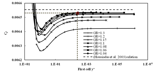
Figure 2 The change of skin coefficient with the first cell y+ at different growth rate values.

Nevertheless, the relation between the relative error and the number of cells required to reach a constant value of Cf at each growth rate is represented in Figure 3 to obtain the optimum growth rate for the present study. The figure shows that the growth rate less than 1.06 with relative error less than 0.36 % reaches to approximately a constant value of relative error. Therefore, from the previous study, the optimum growth rate and value of first cell y + MathType@MTEF@5@5@+= feaagKart1ev2aaatCvAUfeBSjuyZL2yd9gzLbvyNv2CaerbuLwBLn hiov2DGi1BTfMBaeXatLxBI9gBaerbd9wDYLwzYbItLDharqqtubsr 4rNCHbGeaGqiVu0Je9sqqrpepC0xbbL8F4rqqrFfpeea0xe9Lq=Jc9 vqaqpepm0xbba9pwe9Q8fs0=yqaqpepae9pg0FirpepeKkFr0xfr=x fr=xb9adbaqaaeGaciGaaiaabeqaamaabaabaaGcbaqcLbsaqaaaaa aaaaWdbiaadMhal8aadaahaaqabeaajugWa8qacqGHRaWkaaaaaa@39FF@ at the wall were chosen as 1.06 and 0.00378, respectively. Furthermore, the frictional velocity and hence the skin coefficient were compared with experimental data from Dean’s correlation according to the literature 31 as given by Eq.(12). Also, the final results of the present model are compared with the universal log law for velocity profile as illustrated in Figure 4.

Figure 3 The change of relative error with number of cells to yield constant value of according to each growth rate.
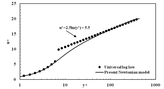
Figure 4 Velocity profile for turbulent channel flow compared with experimental correlation.

u τ = ( 0.073 2 R e m 0.25 U 2 ) MathType@MTEF@5@5@+= feaagKart1ev2aaatCvAUfeBSjuyZL2yd9gzLbvyNv2CaerbuLwBLn hiov2DGi1BTfMBaeXatLxBI9gBaerbd9wDYLwzYbItLDharqqtubsr 4rNCHbGeaGqiVu0Je9sqqrpepC0xbbL8F4rqqrFfpeea0xe9Lq=Jc9 vqaqpepm0xbba9pwe9Q8fs0=yqaqpepae9pg0FirpepeKkFr0xfr=x fr=xb9adbaqaaeGaciGaaiaabeqaamaabaabaaGcbaqcLbsaqaaaaa aaaaWdbiaadwhajuaGpaWaaSbaaSqaaKqzadWdbiabes8a0bWcpaqa baqcLbsapeGaeyypa0tcfa4aaOaaaOWdaeaajuaGpeWaaeWaaOWdae aajuaGpeWaaSaaaOWdaeaajugib8qacaaIWaGaaiOlaiaaicdacaaI 3aGaaG4maaGcpaqaaKqzGeWdbiaaikdaaaGaamOuaiaadwgal8aada WgaaqaaKqzadWdbiaad2gaaSWdaeqaaKqbaoaaCaaaleqabaqcLbsa peGaeyOeI0IaaGimaiaac6cacaaIYaGaaGynaaaacaWGvbWcpaWaaW baaeqabaqcLbmapeGaaGOmaaaaaOGaayjkaiaawMcaaaWcbeaaaaa@5338@ (12)

It is observed from Figure 4 that, the results for the present model agree well with the experimental data which is taken from Dean’s correlation method and both the two curves are indistinguishable on the scale of the figure except for moderate values of y + MathType@MTEF@5@5@+= feaagKart1ev2aaatCvAUfeBSjuyZL2yd9gzLbvyNv2CaerbuLwBLn hiov2DGi1BTfMBaeXatLxBI9gBaerbd9wDYLwzYbItLDharqqtubsr 4rNCHbGeaGqiVu0Je9sqqrpepC0xbbL8F4rqqrFfpeea0xe9Lq=Jc9 vqaqpepm0xbba9pwe9Q8fs0=yqaqpepae9pg0FirpepeKkFr0xfr=x fr=xb9adbaqaaeGaciGaaiaabeqaamaabaabaaGcbaqcLbsaqaaaaa aaaaWdbiaadMhal8aadaahaaqabeaajugWa8qacqGHRaWkaaaaaa@39FF@ . The error at number of cells per height equals 140 is sufficiently small so that this value is considered acceptable for the present study.

Development of approximated k - w model

Traditional model methodology

For turbulent flow, it is more usually to model the Reynolds stresses by Boussinesq approach as described in Eq.(8).26 computed the Reynolds stresses by two-equation models. He introduced the transport equation for k and as represented by Eqs.(9) and (10) for Newtonian fluid. Despite of eddy viscosity for Newtonian fluid is expressed by Eq.(7), it is the most challenge to address for viscoelastic fluids turbulence modeling. Therefore, for drag reducing fluid, the selection of the most adequate expression is of relevant importance to improve the turbulence detection. The most commonly used method for identifying the kinematic eddy viscosity, was developed by25. They modified the eddy viscosity model to be capable of predicting the drag reduction of viscoelastic fluids at different values of Weissenberg numbers. In addition, Resende adapted the kinematic eddy viscosity,  to be the sum of a Newtonian and a polymeric contribution as given by Eq.(13).

ν T =  ν T N ν T p MathType@MTEF@5@5@+= feaagKart1ev2aqatCvAUfeBSjuyZL2yd9gzLbvyNv2CaerbuLwBLn hiov2DGi1BTfMBaeXatLxBI9gBaerbd9wDYLwzYbItLDharqqtubsr 4rNCHbGeaGqiVu0Je9sqqrpepC0xbbL8F4rqqrFfpeea0xe9Lq=Jc9 vqaqpepm0xbba9pwe9Q8fs0=yqaqpepae9pg0FirpepeKkFr0xfr=x fr=xb9adbaqaaeGaciGaaiaabeqaamaabaabaaGcbaqcLbsaqaaaaa aaaaWdbiabe27aULqba+aadaWgaaWcbaqcLbmapeGaamivaaWcpaqa baqcLbsapeGaeyypa0JaaeiOaiabe27aUTWdamaaDaaabaqcLbmape GaamivaaWcpaqaaKqzadWdbiaad6eaaaqcLbsacqGHsislcqaH9oGB l8aadaqhaaqaaKqzadWdbiaadsfaaSWdaeaajugWa8qacaWGWbaaaa aa@4C2A@ (13)

The polymeric contribution to the eddy viscosity, ν T p MathType@MTEF@5@5@+= feaagKart1ev2aqatCvAUfeBSjuyZL2yd9gzLbvyNv2CaerbuLwBLn hiov2DGi1BTfMBaeXatLxBI9gBaerbd9wDYLwzYbItLDharqqtubsr 4rNCHbGeaGqiVu0Je9sqqrpepC0xbbL8F4rqqrFfpeea0xe9Lq=Jc9 vqaqpepm0xbba9pwe9Q8fs0=yqaqpepae9pg0FirpepeKkFr0xfr=x fr=xb9adbaqaaeGaciGaaiaabeqaamaabaabaaGcbaqcLbsaqaaaaa aaaaWdbiabe27aUTWdamaaDaaabaqcLbmapeGaamivaaWcpaqaaKqz adWdbiaadchaaaaaaa@3CFE@ is dependent on the trace of the conformation tensor, C mm MathType@MTEF@5@5@+= feaagKart1ev2aqatCvAUfeBSjuyZL2yd9gzLbvyNv2CaerbuLwBLn hiov2DGi1BTfMBaeXatLxBI9gBaerbd9wDYLwzYbItLDharqqtubsr 4rNCHbGeaGqiVu0Je9sqqrpepC0xbbL8F4rqqrFfpeea0xe9Lq=Jc9 vqaqpepm0xbba9pwe9Q8fs0=yqaqpepae9pg0FirpepeKkFr0xfr=x fr=xb9adbaqaaeGaciGaaiaabeqaamaabaabaaGcbaqcLbsaqaaaaa aaaaWdbiaadoeal8aadaWgaaqaaKqzadWdbiaad2gacaWGTbaal8aa beaaaaa@3AE5@ and introduces a damping function which is relevance to both of Weissenberg number and distance from the wall, i.e., f( W e τo , y + ) MathType@MTEF@5@5@+= feaagKart1ev2aqatCvAUfeBSjuyZL2yd9gzLbvyNv2CaerbuLwBLn hiov2DGi1BTfMBaeXatLxBI9gBaerbd9wDYLwzYbItLDharqqtubsr 4rNCHbGeaGqiVu0Je9sqqrpepC0xbbL8F4rqqrFfpeea0xe9Lq=Jc9 vqaqpepm0xbba9pwe9Q8fs0=yqaqpepae9pg0FirpepeKkFr0xfr=x fr=xb9adbaqaaeGaciGaaiaabeqaamaabaabaaGcbaqcLbsaqaaaaa aaaaWdbiaadAgajuaGdaqadaGcpaqaaKqzGeWdbiaadEfacaWGLbqc fa4damaaBaaaleaajugWa8qacqaHepaDcaWGVbaal8aabeaajugib8 qacaGGSaGaamyEaSWdamaaCaaabeqaaKqzadWdbiabgUcaRaaaaOGa ayjkaiaawMcaaaaa@45B3@ .

ν T p =f( W e τo , y + )× C mm L 2 × C μ × f μ × k ω N MathType@MTEF@5@5@+= feaagKart1ev2aqatCvAUfeBSjuyZL2yd9gzLbvyNv2CaerbuLwBLn hiov2DGi1BTfMBaeXatLxBI9gBaerbd9wDYLwzYbItLDharqqtubsr 4rNCHbGeaGqiVu0Je9sqqrpepC0xbbL8F4rqqrFfpeea0xe9Lq=Jc9 vqaqpepm0xbba9pwe9Q8fs0=yqaqpepae9pg0FirpepeKkFr0xfr=x fr=xb9adbaqaaeGaciGaaiaabeqaamaabaabaaGcbaqcLbsaqaaaaa aaaaWdbiabe27aUTWdamaaDaaabaqcLbmapeGaamivaaWcpaqaaKqz adWdbiaadchaaaqcLbsacqGH9aqpcaWGMbqcfa4aaeWaaOWdaeaaju gib8qacaWGxbGaamyzaKqba+aadaWgaaWcbaqcLbmapeGaeqiXdqNa am4BaaWcpaqabaqcLbsapeGaaiilaiaadMhajuaGpaWaaWbaaSqabe aajugWa8qacqGHRaWkaaaakiaawIcacaGLPaaajugibiabgEna0Mqb aoaalaaak8aabaqcLbsapeGaam4qaKqba+aadaWgaaWcbaqcLbmape GaamyBaiaad2gaaSWdaeqaaaGcbaqcfa4dbmaakaaak8aabaqcLbsa peGaamitaKqba+aadaahaaWcbeqaaKqzadWdbiaaikdaaaaaleqaaa aajugibiabgEna0kaadoeajuaGpaWaaSbaaSqaaKqzadWdbiabeY7a TbWcpaqabaqcLbsapeGaey41aqRaamOzaKqba+aadaWgaaWcbaqcLb mapeGaeqiVd0gal8aabeaajugib8qacqGHxdaTjuaGdaWcaaGcpaqa aKqzGeWdbiaadUgaaOWdaeaajugib8qacqaHjpWDjuaGpaWaaWbaaS qabeaajugWa8qacaWGobaaaaaaaaa@7520@ (14)

Where:

f( W e τo , y + )= C μ p × f μ p × f DR MathType@MTEF@5@5@+= feaagKart1ev2aqatCvAUfeBSjuyZL2yd9gzLbvyNv2CaerbuLwBLn hiov2DGi1BTfMBaeXatLxBI9gBaerbd9wDYLwzYbItLDharqqtubsr 4rNCHbGeaGqiVu0Je9sqqrpepC0xbbL8F4rqqrFfpeea0xe9Lq=Jc9 vqaqpepm0xbba9pwe9Q8fs0=yqaqpepae9pg0FirpepeKkFr0xfr=x fr=xb9adbaqaaeGaciGaaiaabeqaamaabaabaaGcbaqcLbsaqaaaaa aaaaWdbiaadAgajuaGdaqadaGcpaqaaKqzGeWdbiaadEfacaWGLbqc fa4damaaBaaaleaajugWa8qacqaHepaDcaWGVbaal8aabeaajugib8 qacaGGSaGaamyEaKqba+aadaahaaWcbeqaaKqzadWdbiabgUcaRaaa aOGaayjkaiaawMcaaKqzGeGaeyypa0Jaam4qaSWdamaaDaaabaqcLb mapeGaeqiVd0gal8aabaqcLbmapeGaamiCaaaajugibiabgEna0kaa dAgal8aadaqhaaqaaKqzadWdbiabeY7aTbWcpaqaaKqzadWdbiaadc haaaqcLbsacqGHxdaTcaWGMbqcfa4damaaBaaaleaajugWa8qacaWG ebGaamOuaaWcpaqabaaaaa@5E7B@ (15)

C μ p =0.0135× [ 25 W e τo ] 0.12 MathType@MTEF@5@5@+= feaagKart1ev2aqatCvAUfeBSjuyZL2yd9gzLbvyNv2CaerbuLwBLn hiov2DGi1BTfMBaeXatLxBI9gBaerbd9wDYLwzYbItLDharqqtubsr 4rNCHbGeaGqiVu0Je9sqqrpepC0xbbL8F4rqqrFfpeea0xe9Lq=Jc9 vqaqpepm0xbba9pwe9Q8fs0=yqaqpepae9pg0FirpepeKkFr0xfr=x fr=xb9adbaqaaeGaciGaaiaabeqaamaabaabaaGcbaqcLbsaqaaaaa aaaaWdbiaadoeal8aadaqhaaqaaKqzadWdbiabeY7aTbWcpaqaaKqz adWdbiaadchaaaqcLbsacqGH9aqpcaaIWaGaaiOlaiaaicdacaaIXa GaaG4maiaaiwdacqGHxdaTjuaGdaWadaGcpaqaaKqba+qadaWcaaGc paqaaKqzGeWdbiaaikdacaaI1aaak8aabaqcLbsapeGaam4vaiaadw gal8aadaWgaaqaaKqzadWdbiabes8a0jaad+gaaSWdaeqaaaaaaOWd biaawUfacaGLDbaal8aadaahaaqabeaajugWa8qacaaIWaGaaiOlai aaigdacaaIYaaaaaaa@55AF@ (16)

f μ p =[ 1+2.55×exp( y + 44 ) ] MathType@MTEF@5@5@+= feaagKart1ev2aqatCvAUfeBSjuyZL2yd9gzLbvyNv2CaerbuLwBLn hiov2DGi1BTfMBaeXatLxBI9gBaerbd9wDYLwzYbItLDharqqtubsr 4rNCHbGeaGqiVu0Je9sqqrpepC0xbbL8F4rqqrFfpeea0xe9Lq=Jc9 vqaqpepm0xbba9pwe9Q8fs0=yqaqpepae9pg0FirpepeKkFr0xfr=x fr=xb9adbaqaaeGaciGaaiaabeqaamaabaabaaGcbaqcLbsaqaaaaa aaaaWdbiaadAgal8aadaqhaaqaaKqzadWdbiabeY7aTbWcpaqaaKqz adWdbiaadchaaaqcLbsacqGH9aqpjuaGdaWadaGcpaqaaKqzGeWdbi aaigdacqGHRaWkcaaIYaGaaiOlaiaaiwdacaaI1aGaey41aqRaciyz aiaacIhacaGGWbqcfa4aaeWaaOWdaeaajugib8qacqGHsisljuaGda WcaaGcpaqaaKqzGeWdbiaadMhal8aadaahaaqabeaajugWa8qacqGH RaWkaaaak8aabaqcLbsapeGaaGinaiaaisdaaaaakiaawIcacaGLPa aaaiaawUfacaGLDbaaaaa@5600@ (17)

f DR = [ 1exp( W e τo 6.25 ) ] 4 MathType@MTEF@5@5@+= feaagKart1ev2aqatCvAUfeBSjuyZL2yd9gzLbvyNv2CaerbuLwBLn hiov2DGi1BTfMBaeXatLxBI9gBaerbd9wDYLwzYbItLDharqqtubsr 4rNCHbGeaGqiVu0Je9sqqrpepC0xbbL8F4rqqrFfpeea0xe9Lq=Jc9 vqaqpepm0xbba9pwe9Q8fs0=yqaqpepae9pg0FirpepeKkFr0xfr=x fr=xb9adbaqaaeGaciGaaiaabeqaamaabaabaaGcbaqcLbsaqaaaaa aaaaWdbiaadAgajuaGpaWaaSbaaSqaaKqzadWdbiaadseacaWGsbaa l8aabeaajugib8qacqGH9aqpjuaGdaWadaGcpaqaaKqzGeWdbiaaig dacqGHsislciGGLbGaaiiEaiaacchajuaGdaqadaGcpaqaaKqzGeWd biabgkHiTKqbaoaalaaak8aabaqcLbsapeGaam4vaiaadwgal8aada WgaaqaaKqzadWdbiabes8a0jaad+gaaSWdaeqaaaGcbaqcLbsapeGa aGOnaiaac6cacaaIYaGaaGynaaaaaOGaayjkaiaawMcaaaGaay5wai aaw2faaSWdamaaCaaabeqaaKqzadWdbiaaisdaaaaaaa@55AE@ (18)

New methodology description

In the present work, a new average eddy viscosity is supposed, v ˜ T MathType@MTEF@5@5@+= feaagKart1ev2aqatCvAUfeBSjuyZL2yd9gzLbvyNv2CaerbuLwBLn hiov2DGi1BTfMBaeXatLxBI9gBaerbd9wDYLwzYbItLDharqqtubsr 4rNCHbGeaGqiVu0Je9sqqrpepC0xbbL8F4rqqrFfpeea0xe9Lq=Jc9 vqaqpepm0xbba9pwe9Q8fs0=yqaqpepae9pg0FirpepeKkFr0xfr=x fr=xb9adbaqaaeGaciGaaiaabeqaamaabaabaaGcbaGabmODayaaia WaaSbaaSqaaiaadsfaaeqaaaaa@3806@ (based on Resende model), is derived and written in the following expression:

v ˜ T =  ν T N ( 1 ν T p ν T N   ) MathType@MTEF@5@5@+= feaagKart1ev2aqatCvAUfeBSjuyZL2yd9gzLbvyNv2CaerbuLwBLn hiov2DGi1BTfMBaeXatLxBI9gBaerbd9wDYLwzYbItLDharqqtubsr 4rNCHbGeaGqiVu0Je9sqqrpepC0xbbL8F4rqqrFfpeea0xe9Lq=Jc9 vqaqpepm0xbba9pwe9Q8fs0=yqaqpepae9pg0FirpepeKkFr0xfr=x fr=xb9adbaqaaeGaciGaaiaabeqaamaabaabaaGcbaqcLbsaqaaaaa aaaaWdbiqadAhagaacaKqbaoaaBaaabaqcLbmacaWGubaajuaGbeaa jugibiabg2da9iaabckacqaH9oGBl8aadaqhaaqaaKqzadWdbiaads faaSWdaeaajugWa8qacaWGobaaaKqbaoaabmaak8aabaqcLbsapeGa aGymaiabgkHiTKqbaoaalaaak8aabaqcLbsapeGaeqyVd42cpaWaa0 baaeaajugWa8qacaWGubaal8aabaqcLbmapeGaamiCaaaaaOWdaeaa jugib8qacqaH9oGBl8aadaqhaaqaaKqzadWdbiaadsfaaSWdaeaaju gWa8qacaWGobaaaaaajugibiaabckaaOGaayjkaiaawMcaaaaa@58B1@ (19)

17 approved that there are four parameters that influence DR namely, the Weissenberg number ( W e τo ) MathType@MTEF@5@5@+= feaagKart1ev2aqatCvAUfeBSjuyZL2yd9gzLbvyNv2CaerbuLwBLn hiov2DGi1BTfMBaeXatLxBI9gBaerbd9wDYLwzYbItLDharqqtubsr 4rNCHbGeaGqiVu0Je9sqqrpepC0xbbL8F4rqqrFfpeea0xe9Lq=Jc9 vqaqpepm0xbba9pwe9Q8fs0=yqaqpepae9pg0FirpepeKkFr0xfr=x fr=xb9adbaqaaeGaciGaaiaabeqaamaabaabaaGcbaqcfaieaaaaaa aaa8qadaqadaGcpaqaaKqzGeWdbiaadEfacaWGLbqcfa4damaaBaaa leaajugWa8qacqaHepaDcaWGVbaal8aabeaaaOWdbiaawIcacaGLPa aaaaa@3FA0@ ,the molecular flexibility ( L 2 ) MathType@MTEF@5@5@+= feaagKart1ev2aqatCvAUfeBSjuyZL2yd9gzLbvyNv2CaerbuLwBLn hiov2DGi1BTfMBaeXatLxBI9gBaerbd9wDYLwzYbItLDharqqtubsr 4rNCHbGeaGqiVu0Je9sqqrpepC0xbbL8F4rqqrFfpeea0xe9Lq=Jc9 vqaqpepm0xbba9pwe9Q8fs0=yqaqpepae9pg0FirpepeKkFr0xfr=x fr=xb9adbaqaaeGaciGaaiaabeqaamaabaabaaGcbaqcLbsaqaaaaa aaaaWdbiaacIcacaWGmbWcpaWaaWbaaeqabaqcLbmapeGaaGOmaaaa jugibiaacMcaaaa@3B95@ , the viscosity Ratio ( β ) MathType@MTEF@5@5@+= feaagKart1ev2aqatCvAUfeBSjuyZL2yd9gzLbvyNv2CaerbuLwBLn hiov2DGi1BTfMBaeXatLxBI9gBaerbd9wDYLwzYbItLDharqqtubsr 4rNCHbGeaGqiVu0Je9sqqrpepC0xbbL8F4rqqrFfpeea0xe9Lq=Jc9 vqaqpepm0xbba9pwe9Q8fs0=yqaqpepae9pg0FirpepeKkFr0xfr=x fr=xb9adbaqaaeGaciGaaiaabeqaamaabaabaaGcbaqcfaieaaaaaa aaa8qadaqadaGcpaqaaKqzGeWdbiabek7aIbGccaGLOaGaayzkaaaa aa@3A91@ and the frictional Reynolds number ( R e τ ) MathType@MTEF@5@5@+= feaagKart1ev2aqatCvAUfeBSjuyZL2yd9gzLbvyNv2CaerbuLwBLn hiov2DGi1BTfMBaeXatLxBI9gBaerbd9wDYLwzYbItLDharqqtubsr 4rNCHbGeaGqiVu0Je9sqqrpepC0xbbL8F4rqqrFfpeea0xe9Lq=Jc9 vqaqpepm0xbba9pwe9Q8fs0=yqaqpepae9pg0FirpepeKkFr0xfr=x fr=xb9adbaqaaeGaciGaaiaabeqaamaabaabaaGcbaqcfaieaaaaaa aaa8qadaqadaGcpaqaaKqzGeWdbiaadkfacaWGLbWcpaWaaSbaaeaa jugWa8qacqaHepaDaSWdaeqaaaGcpeGaayjkaiaawMcaaaaa@3E19@ . Consequently, the trace of conformation tensor in Resende damping function is replaced with a new function ( M we ) MathType@MTEF@5@5@+= feaagKart1ev2aqatCvAUfeBSjuyZL2yd9gzLbvyNv2CaerbuLwBLn hiov2DGi1BTfMBaeXatLxBI9gBaerbd9wDYLwzYbItLDharqqtubsr 4rNCHbGeaGqiVu0Je9sqqrpepC0xbbL8F4rqqrFfpeea0xe9Lq=Jc9 vqaqpepm0xbba9pwe9Q8fs0=yqaqpepae9pg0FirpepeKkFr0xfr=x fr=xb9adbaqaaeGaciGaaiaabeqaamaabaabaaGcbaqcfaieaaaaaa aaa8qadaqadaGcpaqaaKqzGeWdbiaad2eal8aadaWgaaqaaKqzadWd biaadEhacaWGLbaal8aabeaaaOWdbiaawIcacaGLPaaaaaa@3D4B@ which has a direct dependency on the previous four parameters. Therefore, the new derived average eddy viscosity v ˜ T MathType@MTEF@5@5@+= feaagKart1ev2aaatCvAUfeBSjuyZL2yd9gzLbvyNv2CaerbuLwBLn hiov2DGi1BTfMBaeXatLxBI9gBaerbd9wDYLwzYbItLDharqqtubsr 4rNCHbGeaGqiVu0Je9sqqrpepC0xbbL8F4rqqrFfpeea0xe9Lq=Jc9 vqaqpepm0xbba9pwe9Q8fs0=yqaqpepae9pg0FirpepeKkFr0xfr=x fr=xb9adbaqaaeGaciGaaiaabeqaamaabaabaaGcbaqcLbsaceWG2b GbaGaajuaGdaWgaaWcbaWaaSbaaWqaaKqzadGaamivaaadbeaaaSqa baaaaa@3A94@ can be expressed as the form of Eq.(14) and is presented by Eq. (20). The new supposed average eddy viscosity ( v ˜ T ) MathType@MTEF@5@5@+= feaagKart1ev2aaatCvAUfeBSjuyZL2yd9gzLbvyNv2CaerbuLwBLn hiov2DGi1BTfMBaeXatLxBI9gBaerbd9wDYLwzYbItLDharqqtubsr 4rNCHbGeaGqiVu0Je9sqqrpepC0xbbL8F4rqqrFfpeea0xe9Lq=Jc9 vqaqpepm0xbba9pwe9Q8fs0=yqaqpepae9pg0FirpepeKkFr0xfr=x fr=xb9adbaqaaeGaciGaaiaabeqaamaabaabaaGcbaqcLbsacaGGOa GabmODayaaiaqcfa4aaSbaaSqaamaaBaaameaajugWaiaadsfaaWqa baaaleqaaKqzGeGaaiykaaaa@3C7C@ is set to depend on both of Resende function, f(W e τo , y + ) MathType@MTEF@5@5@+= feaagKart1ev2aaatCvAUfeBSjuyZL2yd9gzLbvyNv2CaerbuLwBLn hiov2DGi1BTfMBaeXatLxBI9gBaerbd9wDYLwzYbItLDharqqtubsr 4rNCHbGeaGqiVu0Je9sqqrpepC0xbbL8F4rqqrFfpeea0xe9Lq=Jc9 vqaqpepm0xbba9pwe9Q8fs0=yqaqpepae9pg0FirpepeKkFr0xfr=x fr=xb9adbaqaaeGaciGaaiaabeqaamaabaabaaGcbaqcLbsaqaaaaa aaaaWdbiaadAgacaGGOaGaam4vaiaadwgajuaGdaWgaaWcbaqcLbma cqaHepaDcaWGVbaaleqaaKqzGeGaaiilaiaadMhajuaGpaWaaWbaaS qabeaajugib8qacqGHRaWkaaGaaiykaaaa@43E3@ , and M we MathType@MTEF@5@5@+= feaagKart1ev2aaatCvAUfeBSjuyZL2yd9gzLbvyNv2CaerbuLwBLn hiov2DGi1BTfMBaeXatLxBI9gBaerbd9wDYLwzYbItLDharqqtubsr 4rNCHbGeaGqiVu0Je9sqqrpepC0xbbL8F4rqqrFfpeea0xe9Lq=Jc9 vqaqpepm0xbba9pwe9Q8fs0=yqaqpepae9pg0FirpepeKkFr0xfr=x fr=xb9adbaqaaeGaciGaaiaabeqaamaabaabaaGcbaqcLbsaqaaaaa aaaaWdbiaad2eajuaGpaWaaSbaaSqaaKqzadWdbiaadEhacaWGLbaa l8aabeaaaaa@3B7E@ function.

v ˜ T =  ν T N ( 1f( W e τo , y + )× M we   ) MathType@MTEF@5@5@+= feaagKart1ev2aaatCvAUfeBSjuyZL2yd9gzLbvyNv2CaerbuLwBLn hiov2DGi1BTfMBaeXatLxBI9gBaerbd9wDYLwzYbItLDharqqtubsr 4rNCHbGeaGqiVu0Je9sqqrpepC0xbbL8F4rqqrFfpeea0xe9Lq=Jc9 vqaqpepm0xbba9pwe9Q8fs0=yqaqpepae9pg0FirpepeKkFr0xfr=x fr=xb9adbaqaaeGaciGaaiaabeqaamaabaabaaGcbaqcLbsaqaaaaa aaaaWdbiqadAhagaacaKqbaoaaBaaaleaajugWaiaadsfaaSqabaqc LbsacqGH9aqpcaqGGcGaeqyVd42cpaWaa0baaeaajugWa8qacaWGub aal8aabaqcLbmapeGaamOtaaaajuaGdaqadaGcpaqaaKqzGeWdbiaa igdacqGHsislcaWGMbqcfa4aaeWaaOWdaeaajugib8qacaWGxbGaam yzaSWdamaaBaaabaqcLbmapeGaeqiXdqNaam4BaaWcpaqabaqcLbsa peGaaiilaiaadMhajuaGpaWaaWbaaSqabeaajugWa8qacqGHRaWkaa aakiaawIcacaGLPaaajugibiabgEna0kaad2eajuaGpaWaaSbaaSqa aKqzadWdbiaadEhacaWGLbaal8aabeaajugib8qacaqGGcaakiaawI cacaGLPaaaaaa@6038@ (20)

Enhanced new  function and UDF code verification

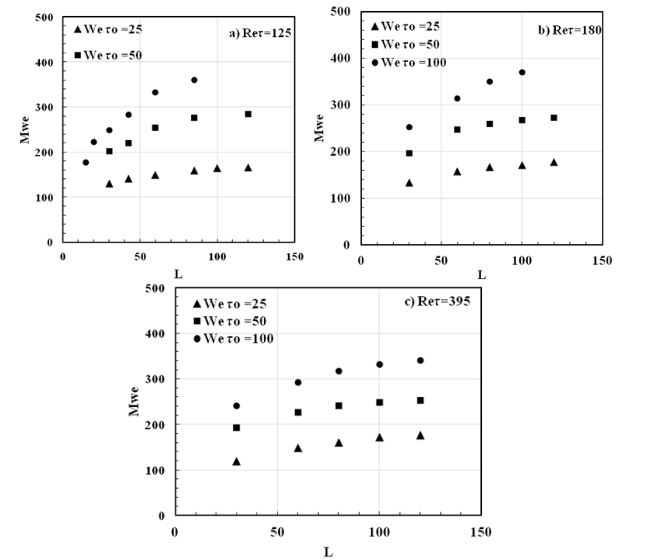
The values of M we MathType@MTEF@5@5@+= feaagKart1ev2aaatCvAUfeBSjuyZL2yd9gzLbvyNv2CaerbuLwBLn hiov2DGi1BTfMBaeXatLxBI9gBaerbd9wDYLwzYbItLDharqqtubsr 4rNCHbGeaGqiVu0Je9sqqrpepC0xbbL8F4rqqrFfpeea0xe9Lq=Jc9 vqaqpepm0xbba9pwe9Q8fs0=yqaqpepae9pg0FirpepeKkFr0xfr=x fr=xb9adbaqaaeGaciGaaiaabeqaamaabaabaaGcbaqcLbsaqaaaaa aaaaWdbiaab2eajuaGpaWaaSbaaSqaaKqzadWdbiaabEhacaqGLbaa l8aabeaaaaa@3B78@ are calculated at different values of maximum extensibility parameter (L) at three different values equal to 25, 50, and 100 of Weissenberg number (W e τo ) MathType@MTEF@5@5@+= feaagKart1ev2aaatCvAUfeBSjuyZL2yd9gzLbvyNv2CaerbuLwBLn hiov2DGi1BTfMBaeXatLxBI9gBaerbd9wDYLwzYbItLDharqqtubsr 4rNCHbGeaGqiVu0Je9sqqrpepC0xbbL8F4rqqrFfpeea0xe9Lq=Jc9 vqaqpepm0xbba9pwe9Q8fs0=yqaqpepae9pg0FirpepeKkFr0xfr=x fr=xb9adbaqaaeGaciGaaiaabeqaamaabaabaaGcbaqcLbsacaGGOa aeaaaaaaaaa8qacaWGxbGaamyzaKqba+aadaWgaaWcbaqcLbmapeGa eqiXdqNaam4BaaWcpaqabaqcLbsacaGGPaaaaa@3F2D@ . Moreover, the results are explored as well to three different 〖Re〗_τ, values equal to 125, 180, and 395 for dilute solution ( β1 ) MathType@MTEF@5@5@+= feaagKart1ev2aaatCvAUfeBSjuyZL2yd9gzLbvyNv2CaerbuLwBLn hiov2DGi1BTfMBaeXatLxBI9gBaerbd9wDYLwzYbItLDharqqtubsr 4rNCHbGeaGqiVu0Je9sqqrpepC0xbbL8F4rqqrFfpeea0xe9Lq=Jc9 vqaqpepm0xbba9pwe9Q8fs0=yqaqpepae9pg0FirpepeKkFr0xfr=x fr=xb9adbaqaaeGaciGaaiaabeqaamaabaabaaGcbaqcfaieaaaaaa aaa8qadaqadaGcpaqaaKqzGeWdbiabek7aIjabloKi7iaaigdaaOGa ayjkaiaawMcaaaaa@3C7C@ . The values of M we MathType@MTEF@5@5@+= feaagKart1ev2aaatCvAUfeBSjuyZL2yd9gzLbvyNv2CaerbuLwBLn hiov2DGi1BTfMBaeXatLxBI9gBaerbd9wDYLwzYbItLDharqqtubsr 4rNCHbGeaGqiVu0Je9sqqrpepC0xbbL8F4rqqrFfpeea0xe9Lq=Jc9 vqaqpepm0xbba9pwe9Q8fs0=yqaqpepae9pg0FirpepeKkFr0xfr=x fr=xb9adbaqaaeGaciGaaiaabeqaamaabaabaaGcbaqcLbsaqaaaaa aaaaWdbiaab2eajuaGpaWaaSbaaSqaaKqzadWdbiaabEhacaqGLbaa l8aabeaaaaa@3B78@ are selected to obtain the same values of DNS drag reduction modeling by using Resende eddy viscosity Model. UDF code is interpreted to ANSYS-Fluent 16.1 solver and Newtonian turbulent viscosity replaced with average turbulent viscosity as represented by Eq.(20). Figure 5 shows the variations of M_we values with the maximum extensibility parameter, L, for three various values of 〖We〗_τo equal to 25, 50, and 150 at three different values of 〖Re〗_τ equal to 125, 180 and 395.It is seen that, for a given values of W e τo MathType@MTEF@5@5@+= feaagKart1ev2aaatCvAUfeBSjuyZL2yd9gzLbvyNv2CaerbuLwBLn hiov2DGi1BTfMBaeXatLxBI9gBaerbd9wDYLwzYbItLDharqqtubsr 4rNCHbGeaGqiVu0Je9sqqrpepC0xbbL8F4rqqrFfpeea0xe9Lq=Jc9 vqaqpepm0xbba9pwe9Q8fs0=yqaqpepae9pg0FirpepeKkFr0xfr=x fr=xb9adbaqaaeGaciGaaiaabeqaamaabaabaaGcbaqcLbsaqaaaaa aaaaWdbiaadEfacaWGLbqcfa4damaaBaaaleaajugWa8qacqaHepaD caWGVbaal8aabeaaaaa@3D45@ and R e τ MathType@MTEF@5@5@+= feaagKart1ev2aaatCvAUfeBSjuyZL2yd9gzLbvyNv2CaerbuLwBLn hiov2DGi1BTfMBaeXatLxBI9gBaerbd9wDYLwzYbItLDharqqtubsr 4rNCHbGeaGqiVu0Je9sqqrpepC0xbbL8F4rqqrFfpeea0xe9Lq=Jc9 vqaqpepm0xbba9pwe9Q8fs0=yqaqpepae9pg0FirpepeKkFr0xfr=x fr=xb9adbaqaaeGaciGaaiaabeqaamaabaabaaGcbaqcLbsaqaaaaa aaaaWdbiaadkfacaWGLbqcfa4damaaBaaaleaajugWa8qacqaHepaD aSWdaeqaaaaa@3C4C@ the value of M we MathType@MTEF@5@5@+= feaagKart1ev2aaatCvAUfeBSjuyZL2yd9gzLbvyNv2CaerbuLwBLn hiov2DGi1BTfMBaeXatLxBI9gBaerbd9wDYLwzYbItLDharqqtubsr 4rNCHbGeaGqiVu0Je9sqqrpepC0xbbL8F4rqqrFfpeea0xe9Lq=Jc9 vqaqpepm0xbba9pwe9Q8fs0=yqaqpepae9pg0FirpepeKkFr0xfr=x fr=xb9adbaqaaeGaciGaaiaabeqaamaabaabaaGcbaqcLbsaqaaaaa aaaaWdbiaab2eajuaGpaWaaSbaaSqaaKqzadWdbiaabEhacaqGLbaa l8aabeaaaaa@3B78@ increases with increasing L and eventually asymptotes. Figure 5 also shows that, the effect of varying the value of M we MathType@MTEF@5@5@+= feaagKart1ev2aaatCvAUfeBSjuyZL2yd9gzLbvyNv2CaerbuLwBLn hiov2DGi1BTfMBaeXatLxBI9gBaerbd9wDYLwzYbItLDharqqtubsr 4rNCHbGeaGqiVu0Je9sqqrpepC0xbbL8F4rqqrFfpeea0xe9Lq=Jc9 vqaqpepm0xbba9pwe9Q8fs0=yqaqpepae9pg0FirpepeKkFr0xfr=x fr=xb9adbaqaaeGaciGaaiaabeqaamaabaabaaGcbaqcLbsaqaaaaa aaaaWdbiaab2eajuaGpaWaaSbaaSqaaKqzadWdbiaabEhacaqGLbaa l8aabeaaaaa@3B78@ increases with increasing W e τo MathType@MTEF@5@5@+= feaagKart1ev2aaatCvAUfeBSjuyZL2yd9gzLbvyNv2CaerbuLwBLn hiov2DGi1BTfMBaeXatLxBI9gBaerbd9wDYLwzYbItLDharqqtubsr 4rNCHbGeaGqiVu0Je9sqqrpepC0xbbL8F4rqqrFfpeea0xe9Lq=Jc9 vqaqpepm0xbba9pwe9Q8fs0=yqaqpepae9pg0FirpepeKkFr0xfr=x fr=xb9adbaqaaeGaciGaaiaabeqaamaabaabaaGcbaqcLbsaqaaaaa aaaaWdbiaadEfacaWGLbqcfa4damaaBaaaleaajugWa8qacqaHepaD caWGVbaal8aabeaaaaa@3D45@ , and it decreases with increasing of R e τ MathType@MTEF@5@5@+= feaagKart1ev2aaatCvAUfeBSjuyZL2yd9gzLbvyNv2CaerbuLwBLn hiov2DGi1BTfMBaeXatLxBI9gBaerbd9wDYLwzYbItLDharqqtubsr 4rNCHbGeaGqiVu0Je9sqqrpepC0xbbL8F4rqqrFfpeea0xe9Lq=Jc9 vqaqpepm0xbba9pwe9Q8fs0=yqaqpepae9pg0FirpepeKkFr0xfr=x fr=xb9adbaqaaeGaciGaaiaabeqaamaabaabaaGcbaqcLbsaqaaaaa aaaaWdbiaadkfacaWGLbqcfa4damaaBaaaleaajugWa8qacqaHepaD aSWdaeqaaaaa@3C4C@ at the same value of L and W e τo MathType@MTEF@5@5@+= feaagKart1ev2aaatCvAUfeBSjuyZL2yd9gzLbvyNv2CaerbuLwBLn hiov2DGi1BTfMBaeXatLxBI9gBaerbd9wDYLwzYbItLDharqqtubsr 4rNCHbGeaGqiVu0Je9sqqrpepC0xbbL8F4rqqrFfpeea0xe9Lq=Jc9 vqaqpepm0xbba9pwe9Q8fs0=yqaqpepae9pg0FirpepeKkFr0xfr=x fr=xb9adbaqaaeGaciGaaiaabeqaamaabaabaaGcbaqcLbsaqaaaaa aaaaWdbiaadEfacaWGLbWcpaWaaSbaaeaajugWa8qacqaHepaDcaWG Vbaal8aabeaaaaa@3CB7@ . Consequently, Figure 6 shows the fitting data, in dashed line, by the Least Square Method with minimum value of determination factor, R 2 0.93 MathType@MTEF@5@5@+= feaagKart1ev2aaatCvAUfeBSjuyZL2yd9gzLbvyNv2CaerbuLwBLn hiov2DGi1BTfMBaeXatLxBI9gBaerbd9wDYLwzYbItLDharqqtubsr 4rNCHbGeaGqiVu0Je9sqqrpepC0xbbL8F4rqqrFfpeea0xe9Lq=Jc9 vqaqpepm0xbba9pwe9Q8fs0=yqaqpepae9pg0FirpepeKkFr0xfr=x fr=xb9adbaqaaeGaciGaaiaabeqaamaabaabaaGcbaqcLbsaqaaaaa aaaaWdbiaadkfal8aadaahaaqabeaajugWa8qacaaIYaaaaKqzGeWd aiabloKi78qacaaIWaGaaiOlaiaaiMdacaaIZaaaaa@3E7D@ over the entire range of M we MathType@MTEF@5@5@+= feaagKart1ev2aaatCvAUfeBSjuyZL2yd9gzLbvyNv2CaerbuLwBLn hiov2DGi1BTfMBaeXatLxBI9gBaerbd9wDYLwzYbItLDharqqtubsr 4rNCHbGeaGqiVu0Je9sqqrpepC0xbbL8F4rqqrFfpeea0xe9Lq=Jc9 vqaqpepm0xbba9pwe9Q8fs0=yqaqpepae9pg0FirpepeKkFr0xfr=x fr=xb9adbaqaaeGaciGaaiaabeqaamaabaabaaGcbaqcLbsaqaaaaa aaaaWdbiaab2eajuaGpaWaaSbaaSqaaKqzadWdbiaabEhacaqGLbaa l8aabeaaaaa@3B78@ values resulting in Eq.  with the relevant constants values as following:

M we = a( 1exp( bL ) )×( 1exp( c( W e τo d ) ( R e τ 125 ) e )  ) MathType@MTEF@5@5@+= feaagKart1ev2aaatCvAUfeBSjuyZL2yd9gzLbvyNv2CaerbuLwBLn hiov2DGi1BTfMBaeXatLxBI9gBaerbd9wDYLwzYbItLDharqqtubsr 4rNCHbGeaGqiVu0Je9sqqrpepC0xbbL8F4rqqrFfpeea0xe9Lq=Jc9 vqaqpepm0xbba9pwe9Q8fs0=yqaqpepae9pg0FirpepeKkFr0xfr=x fr=xb9adbaqaaeGaciGaaiaabeqaamaabaabaaGcbaqcLbsaqaaaaa aaaaWdbiaad2eal8aadaWgaaqaaKqzadWdbiaadEhacaWGLbaal8aa beaajugib8qacqGH9aqpcaqGGcGaamyyaKqbaoaabmaak8aabaqcLb sapeGaaGymaiabgkHiTiGacwgacaGG4bGaaiiCaKqbaoaabmaak8aa baqcLbsapeGaeyOeI0IaamOyaiaadYeaaOGaayjkaiaawMcaaaGaay jkaiaawMcaaKqzGeGaey41aqBcfa4aaeWaaOWdaeaajugib8qacaaI XaGaeyOeI0IaciyzaiaacIhacaGGWbqcfa4aaeWaaOWdaeaajugib8 qacqGHsislcaWGJbqcfa4aaeWaaOWdaeaajugib8qacaWGxbGaamyz aSWdamaaBaaabaqcLbmapeGaeqiXdqNaam4BaaWcpaqabaqcLbsape GaeyOeI0IaamizaaGccaGLOaGaayzkaaqcfa4aaeWaaOWdaeaajuaG peWaaSaaaOWdaeaajugib8qacaWGsbGaamyzaKqba+aadaWgaaWcba qcLbmapeGaeqiXdqhal8aabeaaaOqaaKqzGeWdbiaaigdacaaIYaGa aGynaaaaaOGaayjkaiaawMcaaKqba+aadaahaaWcbeqaaKqzadWdbi abgkHiTiaadwgaaaaakiaawIcacaGLPaaajugibiaacckaaOGaayjk aiaawMcaaaaa@7736@ (21)

Where:

a=386.336;  b=0.0425;  c=0.0247;  d=0.0986;  e=0.1157 MathType@MTEF@5@5@+= feaagKart1ev2aaatCvAUfeBSjuyZL2yd9gzLbvyNv2CaerbuLwBLn hiov2DGi1BTfMBaeXatLxBI9gBaerbd9wDYLwzYbItLDharqqtubsr 4rNCHbGeaGqiVu0Je9sqqrpepC0xbbL8F4rqqrFfpeea0xe9Lq=Jc9 vqaqpepm0xbba9pwe9Q8fs0=yqaqpepae9pg0FirpepeKkFr0xfr=x fr=xb9adbaqaaeGaciGaaiaabeqaamaabaabaaGcbaqcLbsaqaaaaa aaaaWdbiaadggacqGH9aqpcaaIZaGaaGioaiaaiAdacaGGUaGaaG4m aiaaiodacaaI2aGaai4oaiaacckakiaacckajugibiaadkgacqGH9a qpcaaIWaGaaiOlaiaaicdacaaI0aGaaGOmaiaaiwdacaGG7aGaaiiO aOGaaiiOaKqzGeGaam4yaiabg2da9iaaicdacaGGUaGaaGimaiaaik dacaaI0aGaaG4naiaacUdacaGGGcGccaGGGcqcLbsacaWGKbGaeyyp a0JaaGimaiaac6cacaaIWaGaaGyoaiaaiIdacaaI2aGaai4oaiaacc kakiaacckajugibiaadwgacqGH9aqpcaaIWaGaaiOlaiaaigdacaaI XaGaaGynaiaaiEdaaaa@6583@

Figure 5 Variation of with maximum extensibility parameter, L, and Weissen berg number equal to 25, 50, 100 at a: R e τ =125 MathType@MTEF@5@5@+= feaagKart1ev2aqatCvAUfeBSjuyZL2yd9gzLbvyNv2CaerbuLwBLn hiov2DGi1BTfMBaeXatLxBI9gBaerbd9wDYLwzYbItLDharqqtubsr 4rNCHbGeaGqiVu0Je9sqqrpepC0xbbL8F4rqqrFfpeea0xe9Lq=Jc9 vqaqpepm0xbba9pwe9Q8fs0=yqaqpepae9pg0FirpepeKkFr0xfr=x fr=xb9adbaqaaeGaciGaaiaabeqaamaabaabaaGcbaqcLbsaqaaaaa aaaaWdbiaadkfacaWGLbqcfa4damaaBaaaleaajugWa8qacqaHepaD aSWdaeqaaKqzGeWdbiabg2da9iaaigdacaaIYaGaaGynaaaa@4028@ ; b: R e τ =180 MathType@MTEF@5@5@+= feaagKart1ev2aqatCvAUfeBSjuyZL2yd9gzLbvyNv2CaerbuLwBLn hiov2DGi1BTfMBaeXatLxBI9gBaerbd9wDYLwzYbItLDharqqtubsr 4rNCHbGeaGqiVu0Je9sqqrpepC0xbbL8F4rqqrFfpeea0xe9Lq=Jc9 vqaqpepm0xbba9pwe9Q8fs0=yqaqpepae9pg0FirpepeKkFr0xfr=x fr=xb9adbaqaaeGaciGaaiaabeqaamaabaabaaGcbaqcLbsaqaaaaa aaaaWdbiaadkfacaWGLbqcfa4damaaBaaaleaajugWa8qacqaHepaD aSWdaeqaaKqzGeWdbiabg2da9iaaigdacaaI4aGaaGimaaaa@4029@ ; c s: R e τ =395 MathType@MTEF@5@5@+= feaagKart1ev2aaatCvAUfeBSjuyZL2yd9gzLbvyNv2CaerbuLwBLn hiov2DGi1BTfMBaeXatLxBI9gBaerbd9wDYLwzYbItLDharqqtubsr 4rNCHbGeaGqiVu0Je9sqqrpepC0xbbL8F4rqqrFfpeea0xe9Lq=Jc9 vqaqpepm0xbba9pwe9Q8fs0=yqaqpepae9pg0FirpepeKkFr0xfr=x fr=xb9adbaqaaeGaciGaaiaabeqaamaabaabaaGcbaqcLbsaqaaaaa aaaaWdbiaadkfacaWGLbqcfa4damaaBaaaleaajugWa8qacqaHepaD aSWdaeqaaKqzGeWdbiabg2da9iaaiodacaaI5aGaaGynaaaa@4030@ .

Figure 6 Fitting data of M_we function with maximum extensibility parameter, L, and Weissenberg number at a: R e τ =125 MathType@MTEF@5@5@+= feaagKart1ev2aqatCvAUfeBSjuyZL2yd9gzLbvyNv2CaerbuLwBLn hiov2DGi1BTfMBaeXatLxBI9gBaerbd9wDYLwzYbItLDharqqtubsr 4rNCHbGeaGqiVu0Je9sqqrpepC0xbbL8F4rqqrFfpeea0xe9Lq=Jc9 vqaqpepm0xbba9pwe9Q8fs0=yqaqpepae9pg0FirpepeKkFr0xfr=x fr=xb9adbaqaaeGaciGaaiaabeqaamaabaabaaGcbaqcLbsaqaaaaa aaaaWdbiaadkfacaWGLbqcfa4damaaBaaaleaajugWa8qacqaHepaD aSWdaeqaaKqzGeWdbiabg2da9iaaigdacaaIYaGaaGynaaaa@4028@ ;b: R e τ =180 MathType@MTEF@5@5@+= feaagKart1ev2aqatCvAUfeBSjuyZL2yd9gzLbvyNv2CaerbuLwBLn hiov2DGi1BTfMBaeXatLxBI9gBaerbd9wDYLwzYbItLDharqqtubsr 4rNCHbGeaGqiVu0Je9sqqrpepC0xbbL8F4rqqrFfpeea0xe9Lq=Jc9 vqaqpepm0xbba9pwe9Q8fs0=yqaqpepae9pg0FirpepeKkFr0xfr=x fr=xb9adbaqaaeGaciGaaiaabeqaamaabaabaaGcbaqcLbsaqaaaaa aaaaWdbiaadkfacaWGLbqcfa4damaaBaaaleaajugWa8qacqaHepaD aSWdaeqaaKqzGeWdbiabg2da9iaaigdacaaI4aGaaGimaaaa@4029@ ;c: R e τ =395 MathType@MTEF@5@5@+= feaagKart1ev2aaatCvAUfeBSjuyZL2yd9gzLbvyNv2CaerbuLwBLn hiov2DGi1BTfMBaeXatLxBI9gBaerbd9wDYLwzYbItLDharqqtubsr 4rNCHbGeaGqiVu0Je9sqqrpepC0xbbL8F4rqqrFfpeea0xe9Lq=Jc9 vqaqpepm0xbba9pwe9Q8fs0=yqaqpepae9pg0FirpepeKkFr0xfr=x fr=xb9adbaqaaeGaciGaaiaabeqaamaabaabaaGcbaqcLbsaqaaaaa aaaaWdbiaadkfacaWGLbqcfa4damaaBaaaleaajugWa8qacqaHepaD aSWdaeqaaKqzGeWdbiabg2da9iaaiodacaaI5aGaaGynaaaa@4030@ .

Results and discussion

The new proposed turbulence model was validated by DNS model for viscoelastic FENE-P fluids in fully developed turbulent channel flow. The simulations were performed for different values of frictional Reynolds number (R e τ ) MathType@MTEF@5@5@+= feaagKart1ev2aaatCvAUfeBSjuyZL2yd9gzLbvyNv2CaerbuLwBLn hiov2DGi1BTfMBaeXatLxBI9gBaerbd9wDYLwzYbItLDharqqtubsr 4rNCHbGeaGqiVu0Je9sqqrpepC0xbbL8F4rqqrFfpeea0xe9Lq=Jc9 vqaqpepm0xbba9pwe9Q8fs0=yqaqpepae9pg0FirpepeKkFr0xfr=x fr=xb9adbaqaaeGaciGaaiaabeqaamaabaabaaGcbaqcLbsaqaaaaa aaaaWdbiaacIcacaWGsbGaamyzaKqba+aadaWgaaWcbaqcLbmapeGa eqiXdqhal8aabeaajugibiaacMcaaaa@3E34@ maximum extensibility parameter of polymer (L) and different values of Weissenberg number (W e τo ) MathType@MTEF@5@5@+= feaagKart1ev2aaatCvAUfeBSjuyZL2yd9gzLbvyNv2CaerbuLwBLn hiov2DGi1BTfMBaeXatLxBI9gBaerbd9wDYLwzYbItLDharqqtubsr 4rNCHbGeaGqiVu0Je9sqqrpepC0xbbL8F4rqqrFfpeea0xe9Lq=Jc9 vqaqpepm0xbba9pwe9Q8fs0=yqaqpepae9pg0FirpepeKkFr0xfr=x fr=xb9adbaqaaeGaciGaaiaabeqaamaabaabaaGcbaqcLbsacaGGOa aeaaaaaaaaa8qacaWGxbGaamyzaKqba+aadaWgaaWcbaqcLbmapeGa eqiXdqNaam4BaaWcpaqabaqcLbsacaGGPaaaaa@3F2D@ . The new investigated model predictions for both of mean velocity profile and turbulent viscosity ratio were compared with the DNS model, Resende kω MathType@MTEF@5@5@+= feaagKart1ev2aaatCvAUfeBSjuyZL2yd9gzLbvyNv2CaerbuLwBLn hiov2DGi1BTfMBaeXatLxBI9gBaerbd9wDYLwzYbItLDharqqtubsr 4rNCHbGeaGqiVu0Je9sqqrpepC0xbbL8F4rqqrFfpeea0xe9Lq=Jc9 vqaqpepm0xbba9pwe9Q8fs0=yqaqpepae9pg0FirpepeKkFr0xfr=x fr=xb9adbaqaaeGaciGaaiaabeqaamaabaabaaGcbaqcLbsaqaaaaa aaaaWdbiaadUgacqGHsislcqaHjpWDaaa@3A4F@ turbulence model and other RANS eddy viscosity models at different values of frictional Reynolds number, Weissenberg number and maximum extension of polymers. Furthermore, the model compared with the experimental results of Warholic M et al.30 at different values of polymer concentration in low, intermediate and higher drag reduction regions for fully-developed turbulent channel flow.

The developed model results validation with DNS

The results of the present turbulence model were validated with the DNS results of Li C et al13 which are based on FENE-P model at all regions of drag reduction (i.e. low, intermediate and high drag reduction). As seen in Table 1, the present model predictions show excellent agreement with the DNS results at low and intermediate drag reduction regions (i.e. DR60 % ) with a maximum error only reaches about 5 %. However, the error increased in some cases due to the discrepancy between the fitted equation points and the actual value of drag reduction such as the case of R e τ =395,  W e τo =100 MathType@MTEF@5@5@+= feaagKart1ev2aaatCvAUfeBSjuyZL2yd9gzLbvyNv2CaerbuLwBLn hiov2DGi1BTfMBaeXatLxBI9gBaerbd9wDYLwzYbItLDharqqtubsr 4rNCHbGeaGqiVu0Je9sqqrpepC0xbbL8F4rqqrFfpeea0xe9Lq=Jc9 vqaqpepm0xbba9pwe9Q8fs0=yqaqpepae9pg0FirpepeKkFr0xfr=x fr=xb9adbaqaaeGaciGaaiaabeqaamaabaabaaGcbaqcLbsaqaaaaa aaaaWdbiaadkfacaWGLbqcfa4damaaBaaaleaajugWa8qacqaHepaD aSWdaeqaaKqzGeWdbiabg2da9iaaiodacaaI5aGaaGynaiaacYcaca GGGcGaaiiOaiaadEfacaWGLbqcfa4damaaBaaaleaajugWa8qacqaH epaDcaWGVbaal8aabeaajugib8qacqGH9aqpcaaIXaGaaGimaiaaic daaaa@4D9C@ and L=60. The discrepancy appears clearly in Figure 7. On the other hand, in the case of high drag reduction region and near Virk’s asymptote, the accuracy of the model is lost as expected.

R e τ MathType@MTEF@5@5@+= feaagKart1ev2aqatCvAUfeBSjuyZL2yd9gzLbvyNv2CaerbuLwBLn hiov2DGi1BTfMBaeXatLxBI9gBaerbd9wDYLwzYbItLDharqqtubsr 4rNCHbGeaGqiVu0Je9sqqrpepC0xbbL8F4rqqrFfpeea0xe9Lq=Jc9 vqaqpepm0xbba9pwe9Q8fs0=yqaqpepae9pg0FirpepeKkFr0xfr=x fr=xb9adbaqaaeGaciGaaiaabeqaamaabaabaaGcbaqcLbsaqaaaaa aaaaWdbiaadkfacaWGLbqcfa4damaaBaaaleaajugWa8qacqaHepaD aSWdaeqaaaaa@3C4D@

L

W e τo MathType@MTEF@5@5@+= feaagKart1ev2aqatCvAUfeBSjuyZL2yd9gzLbvyNv2CaerbuLwBLn hiov2DGi1BTfMBaeXatLxBI9gBaerbd9wDYLwzYbItLDharqqtubsr 4rNCHbGeaGqiVu0Je9sqqrpepC0xbbL8F4rqqrFfpeea0xe9Lq=Jc9 vqaqpepm0xbba9pwe9Q8fs0=yqaqpepae9pg0FirpepeKkFr0xfr=x fr=xb9adbaqaaeGaciGaaiaabeqaamaabaabaaGcbaqcLbsaqaaaaa aaaaWdbiaadEfacaWGLbWcpaWaaSbaaeaajugWa8qacqaHepaDcaWG Vbaal8aabeaaaaa@3CB8@

DNS DR %

Mwe

Model DR %

Relative error %

125

30

25

18.5

128.23

18.23

1.46

30

100

37

255.1

38.4

3.78

60

100

56.5

326.3

56.2

0.53

85

100

69

344.2

59.6

13.62

120

100

74

351.7

60.7

17.97

180

30

25

19

124.4

18.1

4.74

30

100

38.5

252.6

38.73

0.6

60

100

54

323.068

56.67

4.94

120

100

71

348.23

63.29

10.86

395

30

50

30.5

184.179

29.12

4.52

60

100

49

315.46

55

12.24

120

100

61

340.032

61.6

0.98

120

200

75

378.97

63.7

15.07

Table 1 Comparison between the drag reduction predicted by the present model and DNS drag reduction of Li C et al.13

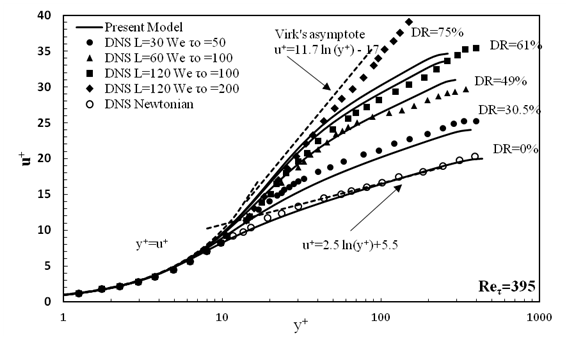
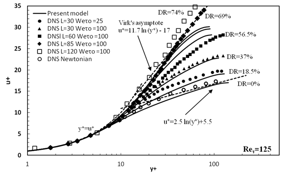
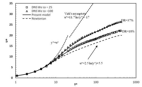
Typical mean velocity profiles as a function of the normalized distance from a wall ( y + ) MathType@MTEF@5@5@+= feaagKart1ev2aaatCvAUfeBSjuyZL2yd9gzLbvyNv2CaerbuLwBLn hiov2DGi1BTfMBaeXatLxBI9gBaerbd9wDYLwzYbItLDharqqtubsr 4rNCHbGeaGqiVu0Je9sqqrpepC0xbbL8F4rqqrFfpeea0xe9Lq=Jc9 vqaqpepm0xbba9pwe9Q8fs0=yqaqpepae9pg0FirpepeKkFr0xfr=x fr=xb9adbaqaaeGaciGaaiaabeqaamaabaabaaGcbaqcfaieaaaaaa aaa8qadaqadaGcpaqaaKqzGeWdbiaadMhal8aadaahaaqabeaajugW a8qacqGHRaWkaaaakiaawIcacaGLPaaaaaa@3C49@ in logarithmic scale in the low, intermediate and high drag reduction regions are shown in Figures 7−9. For the sake of comparison, the mean velocity profiles for Newtonian flow have been included at every Reynolds number.

 For the Newtonian cases, excellent agreement was obtained for the velocity distribution in the viscous sublayer ( u + = y + ) MathType@MTEF@5@5@+= feaagKart1ev2aaatCvAUfeBSjuyZL2yd9gzLbvyNv2CaerbuLwBLn hiov2DGi1BTfMBaeXatLxBI9gBaerbd9wDYLwzYbItLDharqqtubsr 4rNCHbGeaGqiVu0Je9sqqrpepC0xbbL8F4rqqrFfpeea0xe9Lq=Jc9 vqaqpepm0xbba9pwe9Q8fs0=yqaqpepae9pg0FirpepeKkFr0xfr=x fr=xb9adbaqaaeGaciGaaiaabeqaamaabaabaaGcbaqcfaieaaaaaa aaa8qadaqadaGcpaqaaKqzGeWdbiaadwhal8aadaahaaqabeaajugW a8qacqGHRaWkaaqcLbsacqGH9aqpcaWG5bqcfa4damaaCaaaleqaba qcLbmapeGaey4kaScaaaGccaGLOaGaayzkaaaaaa@41C2@ as well as in the log-law layer ( u + =2.5 ln( y + )+5.5 ) MathType@MTEF@5@5@+= feaagKart1ev2aaatCvAUfeBSjuyZL2yd9gzLbvyNv2CaerbuLwBLn hiov2DGi1BTfMBaeXatLxBI9gBaerbd9wDYLwzYbItLDharqqtubsr 4rNCHbGeaGqiVu0Je9sqqrpepC0xbbL8F4rqqrFfpeea0xe9Lq=Jc9 vqaqpepm0xbba9pwe9Q8fs0=yqaqpepae9pg0FirpepeKkFr0xfr=x fr=xb9adbaqaaeGaciGaaiaabeqaamaabaabaaGcbaqcfaieaaaaaa aaa8qadaqadaGcpaqaaKqzGeWdbiaadwhal8aadaahaaqabeaajugW a8qacqGHRaWkaaqcLbsacqGH9aqpcaaIYaGaaiOlaiaaiwdacaGGGc GaamiBaiaad6gajuaGdaqadaGcpaqaaKqzGeWdbiaadMhal8aadaah aaqabeaajugWa8qacqGHRaWkaaaakiaawIcacaGLPaaajugibiabgU caRiaaiwdacaGGUaGaaGynaaGccaGLOaGaayzkaaaaaa@4CE3@ . It can be seen that, all the velocity profiles in the drag reduced flow have the same linear distribution ( u + = y + ) MathType@MTEF@5@5@+= feaagKart1ev2aaatCvAUfeBSjuyZL2yd9gzLbvyNv2CaerbuLwBLn hiov2DGi1BTfMBaeXatLxBI9gBaerbd9wDYLwzYbItLDharqqtubsr 4rNCHbGeaGqiVu0Je9sqqrpepC0xbbL8F4rqqrFfpeea0xe9Lq=Jc9 vqaqpepm0xbba9pwe9Q8fs0=yqaqpepae9pg0FirpepeKkFr0xfr=x fr=xb9adbaqaaeGaciGaaiaabeqaamaabaabaaGcbaqcLbsaqaaaaa aaaaWdbiaacIcacaWG1bWcpaWaaWbaaeqabaqcLbmapeGaey4kaSca aKqzGeGaeyypa0JaamyEaSWdamaaCaaabeqaaKqzadWdbiabgUcaRa aajugibiaacMcaaaa@40D2@ in the viscous sub layer.

Figure 7 Mean velocity profiles predictions compared with the DNS data of 13 for turbulent channel flow with R e τ =395 MathType@MTEF@5@5@+= feaagKart1ev2aaatCvAUfeBSjuyZL2yd9gzLbvyNv2CaerbuLwBLn hiov2DGi1BTfMBaeXatLxBI9gBaerbd9wDYLwzYbItLDharqqtubsr 4rNCHbGeaGqiVu0Je9sqqrpepC0xbbL8F4rqqrFfpeea0xe9Lq=Jc9 vqaqpepm0xbba9pwe9Q8fs0=yqaqpepae9pg0FirpepeKkFr0xfr=x fr=xb9adbaqaaeGaciGaaiaabeqaamaabaabaaGcbaqcLbsaqaaaaa aaaaWdbiaadkfacaWGLbqcfa4damaaBaaaleaajugWa8qacqaHepaD aSWdaeqaaKqzGeWdbiabg2da9iaaiodacaaI5aGaaGynaaaa@4030@ .

Figure 8 Mean velocity profiles predictions compared with the DNS data of13 for turbulent channel flow with R e τ =180 MathType@MTEF@5@5@+= feaagKart1ev2aqatCvAUfeBSjuyZL2yd9gzLbvyNv2CaerbuLwBLn hiov2DGi1BTfMBaeXatLxBI9gBaerbd9wDYLwzYbItLDharqqtubsr 4rNCHbGeaGqiVu0Je9sqqrpepC0xbbL8F4rqqrFfpeea0xe9Lq=Jc9 vqaqpepm0xbba9pwe9Q8fs0=yqaqpepae9pg0FirpepeKkFr0xfr=x fr=xb9adbaqaaeGaciGaaiaabeqaamaabaabaaGcbaqcLbsaqaaaaa aaaaWdbiaadkfacaWGLbqcfa4damaaBaaaleaajugWa8qacqaHepaD aSWdaeqaaKqzGeWdbiabg2da9iaaigdacaaI4aGaaGimaaaa@4029@ .

Figure 9 Mean velocity profiles predictions compared with the DNS data of13 for turbulent channel flow with R e τ =125 MathType@MTEF@5@5@+= feaagKart1ev2aqatCvAUfeBSjuyZL2yd9gzLbvyNv2CaerbuLwBLn hiov2DGi1BTfMBaeXatLxBI9gBaerbd9wDYLwzYbItLDharqqtubsr 4rNCHbGeaGqiVu0Je9sqqrpepC0xbbL8F4rqqrFfpeea0xe9Lq=Jc9 vqaqpepm0xbba9pwe9Q8fs0=yqaqpepae9pg0FirpepeKkFr0xfr=x fr=xb9adbaqaaeGaciGaaiaabeqaamaabaabaaGcbaqcLbsaqaaaaa aaaaWdbiaadkfacaWGLbqcfa4damaaBaaaleaajugWa8qacqaHepaD aSWdaeqaaKqzGeWdbiabg2da9iaaigdacaaIYaGaaGynaaaa@4028@ .

Further away from the wall, specifically in the logarithmic layer, the mean velocity profile increases as compared to that in Newtonian flow. In the low drag reduction region, the profile is shifted upwards with the same slope of Newtonian profile, which is consistent with the experimental results of Warholic M et al.30 In the intermediate and higher drag reduction regions, the slope of the velocity profile in logarithmic layer is increased with increasing the value of the drag reduction until it reaches to the Virk’s asymptote line.

Results of the model against DNS and resende model

The present model was compared with the DNS of Li C et al13 and 25 eddy viscosity models within the turbulent-flow regime at approximately identical frictional Reynolds number R e τ =395 MathType@MTEF@5@5@+= feaagKart1ev2aaatCvAUfeBSjuyZL2yd9gzLbvyNv2CaerbuLwBLn hiov2DGi1BTfMBaeXatLxBI9gBaerbd9wDYLwzYbItLDharqqtubsr 4rNCHbGeaGqiVu0Je9sqqrpepC0xbbL8F4rqqrFfpeea0xe9Lq=Jc9 vqaqpepm0xbba9pwe9Q8fs0=yqaqpepae9pg0FirpepeKkFr0xfr=x fr=xb9adbaqaaeGaciGaaiaabeqaamaabaabaaGcbaqcLbsaqaaaaa aaaaWdbiaadkfacaWGLbWcpaWaaSbaaeaajugWa8qacqaHepaDaSWd aeqaaKqzGeWdbiabg2da9iaaiodacaaI5aGaaGynaaaa@3FA2@ , L=30  MathType@MTEF@5@5@+= feaagKart1ev2aaatCvAUfeBSjuyZL2yd9gzLbvyNv2CaerbuLwBLn hiov2DGi1BTfMBaeXatLxBI9gBaerbd9wDYLwzYbItLDharqqtubsr 4rNCHbGeaGqiVu0Je9sqqrpepC0xbbL8F4rqqrFfpeea0xe9Lq=Jc9 vqaqpepm0xbba9pwe9Q8fs0=yqaqpepae9pg0FirpepeKkFr0xfr=x fr=xb9adbaqaaeGaciGaaiaabeqaamaabaabaaGcbaqcLbsaqaaaaa aaaaWdbiaadYeacqGH9aqpcaaIZaGaaGimaOGaaiiOaaaa@3B21@ and β=0.9 MathType@MTEF@5@5@+= feaagKart1ev2aaatCvAUfeBSjuyZL2yd9gzLbvyNv2CaerbuLwBLn hiov2DGi1BTfMBaeXatLxBI9gBaerbd9wDYLwzYbItLDharqqtubsr 4rNCHbGeaGqiVu0Je9sqqrpepC0xbbL8F4rqqrFfpeea0xe9Lq=Jc9 vqaqpepm0xbba9pwe9Q8fs0=yqaqpepae9pg0FirpepeKkFr0xfr=x fr=xb9adbaqaaeGaciGaaiaabeqaamaabaabaaGcbaqcLbsaqaaaaa aaaaWdbiabek7aIjabg2da9iaaicdacaGGUaGaaGyoaaaa@3B7B@ .

Predicted velocity profile against DNS results and Resende k - w model

Figure 10 demonstrates the predicted data of the mean velocity profile against the DNS results of Li CF et al17{Li, 2006 #2} within the turbulent-flow regime at approximately identical frictional Reynolds number R e τ =395 MathType@MTEF@5@5@+= feaagKart1ev2aaatCvAUfeBSjuyZL2yd9gzLbvyNv2CaerbuLwBLn hiov2DGi1BTfMBaeXatLxBI9gBaerbd9wDYLwzYbItLDharqqtubsr 4rNCHbGeaGqiVu0Je9sqqrpepC0xbbL8F4rqqrFfpeea0xe9Lq=Jc9 vqaqpepm0xbba9pwe9Q8fs0=yqaqpepae9pg0FirpepeKkFr0xfr=x fr=xb9adbaqaaeGaciGaaiaabeqaamaabaabaaGcbaqcLbsaqaaaaa aaaaWdbiaadkfacaWGLbWcpaWaaSbaaeaajugWa8qacqaHepaDaSWd aeqaaKqzGeWdbiabg2da9iaaiodacaaI5aGaaGynaaaa@3FA2@ , L=30  MathType@MTEF@5@5@+= feaagKart1ev2aaatCvAUfeBSjuyZL2yd9gzLbvyNv2CaerbuLwBLn hiov2DGi1BTfMBaeXatLxBI9gBaerbd9wDYLwzYbItLDharqqtubsr 4rNCHbGeaGqiVu0Je9sqqrpepC0xbbL8F4rqqrFfpeea0xe9Lq=Jc9 vqaqpepm0xbba9pwe9Q8fs0=yqaqpepae9pg0FirpepeKkFr0xfr=x fr=xb9adbaqaaeGaciGaaiaabeqaamaabaabaaGcbaqcLbsaqaaaaa aaaaWdbiaadYeacqGH9aqpcaaIZaGaaGimaOGaaiiOaaaa@3B21@ and β=0.9 MathType@MTEF@5@5@+= feaagKart1ev2aaatCvAUfeBSjuyZL2yd9gzLbvyNv2CaerbuLwBLn hiov2DGi1BTfMBaeXatLxBI9gBaerbd9wDYLwzYbItLDharqqtubsr 4rNCHbGeaGqiVu0Je9sqqrpepC0xbbL8F4rqqrFfpeea0xe9Lq=Jc9 vqaqpepm0xbba9pwe9Q8fs0=yqaqpepae9pg0FirpepeKkFr0xfr=x fr=xb9adbaqaaeGaciGaaiaabeqaamaabaabaaGcbaqcLbsaqaaaaa aaaaWdbiabek7aIjabg2da9iaaicdacaGGUaGaaGyoaaaa@3B7B@ . The present model predicted DR=17.1 % MathType@MTEF@5@5@+= feaagKart1ev2aaatCvAUfeBSjuyZL2yd9gzLbvyNv2CaerbuLwBLn hiov2DGi1BTfMBaeXatLxBI9gBaerbd9wDYLwzYbItLDharqqtubsr 4rNCHbGeaGqiVu0Je9sqqrpepC0xbbL8F4rqqrFfpeea0xe9Lq=Jc9 vqaqpepm0xbba9pwe9Q8fs0=yqaqpepae9pg0FirpepeKkFr0xfr=x fr=xb9adbaqaaeGaciGaaiaabeqaamaabaabaaGcbaqcLbsaqaaaaa aaaaWdbiaadseacaWGsbGaeyypa0JaaGymaiaaiEdacaGGUaGaaGym aiaacckacaGGLaaaaa@3E01@ against DR=18 % MathType@MTEF@5@5@+= feaagKart1ev2aaatCvAUfeBSjuyZL2yd9gzLbvyNv2CaerbuLwBLn hiov2DGi1BTfMBaeXatLxBI9gBaerbd9wDYLwzYbItLDharqqtubsr 4rNCHbGeaGqiVu0Je9sqqrpepC0xbbL8F4rqqrFfpeea0xe9Lq=Jc9 vqaqpepm0xbba9pwe9Q8fs0=yqaqpepae9pg0FirpepeKkFr0xfr=x fr=xb9adbaqaaeGaciGaaiaabeqaamaabaabaaGcbaqcLbsaqaaaaa aaaaWdbiaadseacaWGsbGaeyypa0JaaGymaiaaiIdacaGGGcGaaiyj aaaa@3C95@ by DNS results at W e τo =25 MathType@MTEF@5@5@+= feaagKart1ev2aaatCvAUfeBSjuyZL2yd9gzLbvyNv2CaerbuLwBLn hiov2DGi1BTfMBaeXatLxBI9gBaerbd9wDYLwzYbItLDharqqtubsr 4rNCHbGeaGqiVu0Je9sqqrpepC0xbbL8F4rqqrFfpeea0xe9Lq=Jc9 vqaqpepm0xbba9pwe9Q8fs0=yqaqpepae9pg0FirpepeKkFr0xfr=x fr=xb9adbaqaaeGaciGaaiaabeqaamaabaabaaGcbaqcLbsaqaaaaa aaaaWdbiaadEfacaWGLbqcfa4damaaBaaaleaajugWa8qacqaHepaD caWGVbaal8aabeaajugib8qacqGH9aqpcaaIYaGaaGynaaaa@4065@ . Also, at W e τo =100 MathType@MTEF@5@5@+= feaagKart1ev2aaatCvAUfeBSjuyZL2yd9gzLbvyNv2CaerbuLwBLn hiov2DGi1BTfMBaeXatLxBI9gBaerbd9wDYLwzYbItLDharqqtubsr 4rNCHbGeaGqiVu0Je9sqqrpepC0xbbL8F4rqqrFfpeea0xe9Lq=Jc9 vqaqpepm0xbba9pwe9Q8fs0=yqaqpepae9pg0FirpepeKkFr0xfr=x fr=xb9adbaqaaeGaciGaaiaabeqaamaabaabaaGcbaqcLbsaqaaaaa aaaaWdbiaadEfacaWGLbqcfa4damaaBaaaleaajugWa8qacqaHepaD caWGVbaal8aabeaajugib8qacqGH9aqpcaaIXaGaaGimaiaaicdaaa a@4119@ , the present model predicted DR=38.35 % MathType@MTEF@5@5@+= feaagKart1ev2aaatCvAUfeBSjuyZL2yd9gzLbvyNv2CaerbuLwBLn hiov2DGi1BTfMBaeXatLxBI9gBaerbd9wDYLwzYbItLDharqqtubsr 4rNCHbGeaGqiVu0Je9sqqrpepC0xbbL8F4rqqrFfpeea0xe9Lq=Jc9 vqaqpepm0xbba9pwe9Q8fs0=yqaqpepae9pg0FirpepeKkFr0xfr=x fr=xb9adbaqaaeGaciGaaiaabeqaamaabaabaaGcbaqcLbsaqaaaaa aaaaWdbiaadseacaWGsbGaeyypa0JaaG4maiaaiIdacaGGUaGaaG4m aiaaiwdacaGGGcGaaiyjaaaa@3EC5@ against DR=37 % MathType@MTEF@5@5@+= feaagKart1ev2aaatCvAUfeBSjuyZL2yd9gzLbvyNv2CaerbuLwBLn hiov2DGi1BTfMBaeXatLxBI9gBaerbd9wDYLwzYbItLDharqqtubsr 4rNCHbGeaGqiVu0Je9sqqrpepC0xbbL8F4rqqrFfpeea0xe9Lq=Jc9 vqaqpepm0xbba9pwe9Q8fs0=yqaqpepae9pg0FirpepeKkFr0xfr=x fr=xb9adbaqaaeGaciGaaiaabeqaamaabaabaaGcbaqcLbsaqaaaaa aaaaWdbiaadseacaWGsbGaeyypa0JaaG4maiaaiEdacaGGGcGaaiyj aaaa@3C96@ by DNS results. The present model predictions show good agreement with the DNS data specially for the trend of the velocity profile and the values of the drag reduction. The monotonic shift of the log-law region with DR is well captured, as well as the correct evolution in the buffer-layer. In Figure 11, the predicted data of mean velocity profile is compared with the results of both of Resende P et al.25 and DNS models. The Resende model predicted DR=18 % MathType@MTEF@5@5@+= feaagKart1ev2aaatCvAUfeBSjuyZL2yd9gzLbvyNv2CaerbuLwBLn hiov2DGi1BTfMBaeXatLxBI9gBaerbd9wDYLwzYbItLDharqqtubsr 4rNCHbGeaGqiVu0Je9sqqrpepC0xbbL8F4rqqrFfpeea0xe9Lq=Jc9 vqaqpepm0xbba9pwe9Q8fs0=yqaqpepae9pg0FirpepeKkFr0xfr=x fr=xb9adbaqaaeGaciGaaiaabeqaamaabaabaaGcbaqcLbsaqaaaaa aaaaWdbiaadseacaWGsbGaeyypa0JaaGymaiaaiIdacaGGGcGaaiyj aaaa@3C95@ against DR=18 % MathType@MTEF@5@5@+= feaagKart1ev2aaatCvAUfeBSjuyZL2yd9gzLbvyNv2CaerbuLwBLn hiov2DGi1BTfMBaeXatLxBI9gBaerbd9wDYLwzYbItLDharqqtubsr 4rNCHbGeaGqiVu0Je9sqqrpepC0xbbL8F4rqqrFfpeea0xe9Lq=Jc9 vqaqpepm0xbba9pwe9Q8fs0=yqaqpepae9pg0FirpepeKkFr0xfr=x fr=xb9adbaqaaeGaciGaaiaabeqaamaabaabaaGcbaqcLbsaqaaaaa aaaaWdbiaadseacaWGsbGaeyypa0JaaGymaiaaiIdacaGGGcGaaiyj aaaa@3C95@ by DNS and  DR=17 % MathType@MTEF@5@5@+= feaagKart1ev2aaatCvAUfeBSjuyZL2yd9gzLbvyNv2CaerbuLwBLn hiov2DGi1BTfMBaeXatLxBI9gBaerbd9wDYLwzYbItLDharqqtubsr 4rNCHbGeaGqiVu0Je9sqqrpepC0xbbL8F4rqqrFfpeea0xe9Lq=Jc9 vqaqpepm0xbba9pwe9Q8fs0=yqaqpepae9pg0FirpepeKkFr0xfr=x fr=xb9adbaqaaeGaciGaaiaabeqaamaabaabaaGcbaaeaaaaaaaaa8 qacaGGGcqcLbsacaWGebGaamOuaiabg2da9iaaigdacaaI3aGaaiiO aiaacwcaaaa@3DB8@ by the present model results at W e τo =25 MathType@MTEF@5@5@+= feaagKart1ev2aaatCvAUfeBSjuyZL2yd9gzLbvyNv2CaerbuLwBLn hiov2DGi1BTfMBaeXatLxBI9gBaerbd9wDYLwzYbItLDharqqtubsr 4rNCHbGeaGqiVu0Je9sqqrpepC0xbbL8F4rqqrFfpeea0xe9Lq=Jc9 vqaqpepm0xbba9pwe9Q8fs0=yqaqpepae9pg0FirpepeKkFr0xfr=x fr=xb9adbaqaaeGaciGaaiaabeqaamaabaabaaGcbaqcLbsaqaaaaa aaaaWdbiaadEfacaWGLbqcfa4damaaBaaaleaajugWa8qacqaHepaD caWGVbaal8aabeaajugib8qacqGH9aqpcaaIYaGaaGynaaaa@4065@ . Also, at W e τo =100 MathType@MTEF@5@5@+= feaagKart1ev2aaatCvAUfeBSjuyZL2yd9gzLbvyNv2CaerbuLwBLn hiov2DGi1BTfMBaeXatLxBI9gBaerbd9wDYLwzYbItLDharqqtubsr 4rNCHbGeaGqiVu0Je9sqqrpepC0xbbL8F4rqqrFfpeea0xe9Lq=Jc9 vqaqpepm0xbba9pwe9Q8fs0=yqaqpepae9pg0FirpepeKkFr0xfr=x fr=xb9adbaqaaeGaciGaaiaabeqaamaabaabaaGcbaqcLbsaqaaaaa aaaaWdbiaadEfacaWGLbqcfa4damaaBaaaleaajugWa8qacqaHepaD caWGVbaal8aabeaajugib8qacqGH9aqpcaaIXaGaaGimaiaaicdaaa a@4119@ the Resende model predicted DR=39 % MathType@MTEF@5@5@+= feaagKart1ev2aaatCvAUfeBSjuyZL2yd9gzLbvyNv2CaerbuLwBLn hiov2DGi1BTfMBaeXatLxBI9gBaerbd9wDYLwzYbItLDharqqtubsr 4rNCHbGeaGqiVu0Je9sqqrpepC0xbbL8F4rqqrFfpeea0xe9Lq=Jc9 vqaqpepm0xbba9pwe9Q8fs0=yqaqpepae9pg0FirpepeKkFr0xfr=x fr=xb9adbaqaaeGaciGaaiaabeqaamaabaabaaGcbaqcLbsaqaaaaa aaaaWdbiaadseacaWGsbGaeyypa0JaaG4maiaaiMdacaGGGcGaaiyj aaaa@3C98@ against DR=37 % MathType@MTEF@5@5@+= feaagKart1ev2aaatCvAUfeBSjuyZL2yd9gzLbvyNv2CaerbuLwBLn hiov2DGi1BTfMBaeXatLxBI9gBaerbd9wDYLwzYbItLDharqqtubsr 4rNCHbGeaGqiVu0Je9sqqrpepC0xbbL8F4rqqrFfpeea0xe9Lq=Jc9 vqaqpepm0xbba9pwe9Q8fs0=yqaqpepae9pg0FirpepeKkFr0xfr=x fr=xb9adbaqaaeGaciGaaiaabeqaamaabaabaaGcbaqcLbsaqaaaaa aaaaWdbiaadseacaWGsbGaeyypa0JaaG4maiaaiEdacaGGGcGaaiyj aaaa@3C96@ by DNS results and DR=38.35 % MathType@MTEF@5@5@+= feaagKart1ev2aaatCvAUfeBSjuyZL2yd9gzLbvyNv2CaerbuLwBLn hiov2DGi1BTfMBaeXatLxBI9gBaerbd9wDYLwzYbItLDharqqtubsr 4rNCHbGeaGqiVu0Je9sqqrpepC0xbbL8F4rqqrFfpeea0xe9Lq=Jc9 vqaqpepm0xbba9pwe9Q8fs0=yqaqpepae9pg0FirpepeKkFr0xfr=x fr=xb9adbaqaaeGaciGaaiaabeqaamaabaabaaGcbaqcLbsaqaaaaa aaaaWdbiaadseacaWGsbGaeyypa0JaaG4maiaaiIdacaGGUaGaaG4m aiaaiwdacaGGGcGaaiyjaaaa@3EC5@ by the present model.

Figure 10 Comparison between the predictions of the mean velocity by the present model and DNS data of13 for turbulent channel flow with R e τ =395 MathType@MTEF@5@5@+= feaagKart1ev2aqatCvAUfeBSjuyZL2yd9gzLbvyNv2CaerbuLwBLn hiov2DGi1BTfMBaeXatLxBI9gBaerbd9wDYLwzYbItLDharqqtubsr 4rNCHbGeaGqiVu0Je9sqqrpepC0xbbL8F4rqqrFfpeea0xe9Lq=Jc9 vqaqpepm0xbba9pwe9Q8fs0=yqaqpepae9pg0FirpepeKkFr0xfr=x fr=xb9adbaqaaeGaciGaaiaabeqaamaabaabaaGcbaqcLbsaqaaaaa aaaaWdbiaadkfacaWGLbqcfa4damaaBaaaleaajugWa8qacqaHepaD aSWdaeqaaKqzGeWdbiabg2da9iaaiodacaaI5aGaaGynaaaa@4031@ , L=30 MathType@MTEF@5@5@+= feaagKart1ev2aqatCvAUfeBSjuyZL2yd9gzLbvyNv2CaerbuLwBLn hiov2DGi1BTfMBaeXatLxBI9gBaerbd9wDYLwzYbItLDharqqtubsr 4rNCHbGeaGqiVu0Je9sqqrpepC0xbbL8F4rqqrFfpeea0xe9Lq=Jc9 vqaqpepm0xbba9pwe9Q8fs0=yqaqpepae9pg0FirpepeKkFr0xfr=x fr=xb9adbaqaaeGaciGaaiaabeqaamaabaabaaGcbaqcLbsaqaaaaa aaaaWdbiaadYeacqGH9aqpcaaIZaGaaGimaaaa@39F4@ and β=0.9 MathType@MTEF@5@5@+= feaagKart1ev2aaatCvAUfeBSjuyZL2yd9gzLbvyNv2CaerbuLwBLn hiov2DGi1BTfMBaeXatLxBI9gBaerbd9wDYLwzYbItLDharqqtubsr 4rNCHbGeaGqiVu0Je9sqqrpepC0xbbL8F4rqqrFfpeea0xe9Lq=Jc9 vqaqpepm0xbba9pwe9Q8fs0=yqaqpepae9pg0FirpepeKkFr0xfr=x fr=xb9adbaqaaeGaciGaaiaabeqaamaabaabaaGcbaqcLbsaqaaaaa aaaaWdbiabek7aIjabg2da9iaaicdacaGGUaGaaGyoaaaa@3B7B@ at W e τo =25 MathType@MTEF@5@5@+= feaagKart1ev2aaatCvAUfeBSjuyZL2yd9gzLbvyNv2CaerbuLwBLn hiov2DGi1BTfMBaeXatLxBI9gBaerbd9wDYLwzYbItLDharqqtubsr 4rNCHbGeaGqiVu0Je9sqqrpepC0xbbL8F4rqqrFfpeea0xe9Lq=Jc9 vqaqpepm0xbba9pwe9Q8fs0=yqaqpepae9pg0FirpepeKkFr0xfr=x fr=xb9adbaqaaeGaciGaaiaabeqaamaabaabaaGcbaqcLbsaqaaaaa aaaaWdbiaadEfacaWGLbqcfa4damaaBaaaleaajugWa8qacqaHepaD caWGVbaal8aabeaajugib8qacqGH9aqpcaaIYaGaaGynaaaa@4065@ & W e τo =100 MathType@MTEF@5@5@+= feaagKart1ev2aaatCvAUfeBSjuyZL2yd9gzLbvyNv2CaerbuLwBLn hiov2DGi1BTfMBaeXatLxBI9gBaerbd9wDYLwzYbItLDharqqtubsr 4rNCHbGeaGqiVu0Je9sqqrpepC0xbbL8F4rqqrFfpeea0xe9Lq=Jc9 vqaqpepm0xbba9pwe9Q8fs0=yqaqpepae9pg0FirpepeKkFr0xfr=x fr=xb9adbaqaaeGaciGaaiaabeqaamaabaabaaGcbaqcLbsaqaaaaa aaaaWdbiaadEfacaWGLbWcpaWaaSbaaeaajugWa8qacqaHepaDcaWG Vbaal8aabeaajugib8qacqGH9aqpcaaIXaGaaGimaiaaicdaaaa@408B@ .

Figure 11 Comparison between the predictions of the mean velocity by the present model and both DNS model and RANS model of25 for turbulent channel flow with R e τ =395 MathType@MTEF@5@5@+= feaagKart1ev2aqatCvAUfeBSjuyZL2yd9gzLbvyNv2CaerbuLwBLn hiov2DGi1BTfMBaeXatLxBI9gBaerbd9wDYLwzYbItLDharqqtubsr 4rNCHbGeaGqiVu0Je9sqqrpepC0xbbL8F4rqqrFfpeea0xe9Lq=Jc9 vqaqpepm0xbba9pwe9Q8fs0=yqaqpepae9pg0FirpepeKkFr0xfr=x fr=xb9adbaqaaeGaciGaaiaabeqaamaabaabaaGcbaqcLbsaqaaaaa aaaaWdbiaadkfacaWGLbqcfa4damaaBaaaleaajugWa8qacqaHepaD aSWdaeqaaKqzGeWdbiabg2da9iaaiodacaaI5aGaaGynaaaa@4031@ , L=30 MathType@MTEF@5@5@+= feaagKart1ev2aqatCvAUfeBSjuyZL2yd9gzLbvyNv2CaerbuLwBLn hiov2DGi1BTfMBaeXatLxBI9gBaerbd9wDYLwzYbItLDharqqtubsr 4rNCHbGeaGqiVu0Je9sqqrpepC0xbbL8F4rqqrFfpeea0xe9Lq=Jc9 vqaqpepm0xbba9pwe9Q8fs0=yqaqpepae9pg0FirpepeKkFr0xfr=x fr=xb9adbaqaaeGaciGaaiaabeqaamaabaabaaGcbaqcLbsaqaaaaa aaaaWdbiaadYeacqGH9aqpcaaIZaGaaGimaaaa@39F4@ and β=0.9 MathType@MTEF@5@5@+= feaagKart1ev2aaatCvAUfeBSjuyZL2yd9gzLbvyNv2CaerbuLwBLn hiov2DGi1BTfMBaeXatLxBI9gBaerbd9wDYLwzYbItLDharqqtubsr 4rNCHbGeaGqiVu0Je9sqqrpepC0xbbL8F4rqqrFfpeea0xe9Lq=Jc9 vqaqpepm0xbba9pwe9Q8fs0=yqaqpepae9pg0FirpepeKkFr0xfr=x fr=xb9adbaqaaeGaciGaaiaabeqaamaabaabaaGcbaqcLbsaqaaaaa aaaaWdbiabek7aIjabg2da9iaaicdacaGGUaGaaGyoaaaa@3B7B@ at W e τo =25 MathType@MTEF@5@5@+= feaagKart1ev2aaatCvAUfeBSjuyZL2yd9gzLbvyNv2CaerbuLwBLn hiov2DGi1BTfMBaeXatLxBI9gBaerbd9wDYLwzYbItLDharqqtubsr 4rNCHbGeaGqiVu0Je9sqqrpepC0xbbL8F4rqqrFfpeea0xe9Lq=Jc9 vqaqpepm0xbba9pwe9Q8fs0=yqaqpepae9pg0FirpepeKkFr0xfr=x fr=xb9adbaqaaeGaciGaaiaabeqaamaabaabaaGcbaqcLbsaqaaaaa aaaaWdbiaadEfacaWGLbqcfa4damaaBaaaleaajugWa8qacqaHepaD caWGVbaal8aabeaajugib8qacqGH9aqpcaaIYaGaaGynaaaa@4065@ and W e τo =100 MathType@MTEF@5@5@+= feaagKart1ev2aaatCvAUfeBSjuyZL2yd9gzLbvyNv2CaerbuLwBLn hiov2DGi1BTfMBaeXatLxBI9gBaerbd9wDYLwzYbItLDharqqtubsr 4rNCHbGeaGqiVu0Je9sqqrpepC0xbbL8F4rqqrFfpeea0xe9Lq=Jc9 vqaqpepm0xbba9pwe9Q8fs0=yqaqpepae9pg0FirpepeKkFr0xfr=x fr=xb9adbaqaaeGaciGaaiaabeqaamaabaabaaGcbaqcLbsaqaaaaa aaaaWdbiaadEfacaWGLbWcpaWaaSbaaeaajugWa8qacqaHepaDcaWG Vbaal8aabeaajugib8qacqGH9aqpcaaIXaGaaGimaiaaicdaaaa@408B@ .

Predicted eddy viscosity ratio against the DNS and resende k - w model

As seen from Figure 12, the change of the eddy viscosity ratio ( ν T / ν o ) MathType@MTEF@5@5@+= feaagKart1ev2aaatCvAUfeBSjuyZL2yd9gzLbvyNv2CaerbuLwBLn hiov2DGi1BTfMBaeXatLxBI9gBaerbd9wDYLwzYbItLDharqqtubsr 4rNCHbGeaGqiVu0Je9sqqrpepC0xbbL8F4rqqrFfpeea0xe9Lq=Jc9 vqaqpepm0xbba9pwe9Q8fs0=yqaqpepae9pg0FirpepeKkFr0xfr=x fr=xb9adbaqaaeGaciGaaiaabeqaamaabaabaaGcbaqcfaieaaaaaa aaa8qadaqadaGcpaqaaKqzGeWdbiabe27aUTWdamaaBaaabaqcLbma peGaamivaaWcpaqabaqcLbsapeGaai4laiabe27aUTWdamaaBaaaba qcLbmapeGaam4BaaWcpaqabaaak8qacaGLOaGaayzkaaaaaa@42B4@ along y + MathType@MTEF@5@5@+= feaagKart1ev2aaatCvAUfeBSjuyZL2yd9gzLbvyNv2CaerbuLwBLn hiov2DGi1BTfMBaeXatLxBI9gBaerbd9wDYLwzYbItLDharqqtubsr 4rNCHbGeaGqiVu0Je9sqqrpepC0xbbL8F4rqqrFfpeea0xe9Lq=Jc9 vqaqpepm0xbba9pwe9Q8fs0=yqaqpepae9pg0FirpepeKkFr0xfr=x fr=xb9adbaqaaeGaciGaaiaabeqaamaabaabaaGcbaqcLbsaqaaaaa aaaaWdbiaadMhal8aadaahaaqabeaajugWa8qacqGHRaWkaaaaaa@39FF@ is captured especially in the buffer layer region. There is a strong dependency and good agreement of the enhanced predicted eddy viscosities for all studied W e τo MathType@MTEF@5@5@+= feaagKart1ev2aaatCvAUfeBSjuyZL2yd9gzLbvyNv2CaerbuLwBLn hiov2DGi1BTfMBaeXatLxBI9gBaerbd9wDYLwzYbItLDharqqtubsr 4rNCHbGeaGqiVu0Je9sqqrpepC0xbbL8F4rqqrFfpeea0xe9Lq=Jc9 vqaqpepm0xbba9pwe9Q8fs0=yqaqpepae9pg0FirpepeKkFr0xfr=x fr=xb9adbaqaaeGaciGaaiaabeqaamaabaabaaGcbaqcLbsaqaaaaa aaaaWdbiaadEfacaWGLbqcfa4damaaBaaaleaajugWa8qacqaHepaD caWGVbaal8aabeaaaaa@3D45@ values, with DNS eddy viscosities for all y + MathType@MTEF@5@5@+= feaagKart1ev2aaatCvAUfeBSjuyZL2yd9gzLbvyNv2CaerbuLwBLn hiov2DGi1BTfMBaeXatLxBI9gBaerbd9wDYLwzYbItLDharqqtubsr 4rNCHbGeaGqiVu0Je9sqqrpepC0xbbL8F4rqqrFfpeea0xe9Lq=Jc9 vqaqpepm0xbba9pwe9Q8fs0=yqaqpepae9pg0FirpepeKkFr0xfr=x fr=xb9adbaqaaeGaciGaaiaabeqaamaabaabaaGcbaqcLbsaqaaaaa aaaaWdbiaadMhal8aadaahaaqabeaajugWa8qacqGHRaWkaaaaaa@39FF@ range values. The present model is capable to predict the correct evolution shown by the DNS model in the lower and intermediate drag reduction regimes. Furthermore, a DR increment and turbulent viscosity ratio decrement were achieved.

In Figure 13, the predicted turbulent viscosities were compared with DNS and Resende results. This figure also depicted that there is a marked contrast with Resende model for y + MathType@MTEF@5@5@+= feaagKart1ev2aaatCvAUfeBSjuyZL2yd9gzLbvyNv2CaerbuLwBLn hiov2DGi1BTfMBaeXatLxBI9gBaerbd9wDYLwzYbItLDharqqtubsr 4rNCHbGeaGqiVu0Je9sqqrpepC0xbbL8F4rqqrFfpeea0xe9Lq=Jc9 vqaqpepm0xbba9pwe9Q8fs0=yqaqpepae9pg0FirpepeKkFr0xfr=x fr=xb9adbaqaaeGaciGaaiaabeqaamaabaabaaGcbaqcLbsaqaaaaa aaaaWdbiaadMhal8aadaahaaqabeaajugWa8qacqGHRaWkaaaaaa@39FF@ higher values for the same Reynolds number. Therefore, it is clear that the present model predictions coincide with those of Resende model kω MathType@MTEF@5@5@+= feaagKart1ev2aaatCvAUfeBSjuyZL2yd9gzLbvyNv2CaerbuLwBLn hiov2DGi1BTfMBaeXatLxBI9gBaerbd9wDYLwzYbItLDharqqtubsr 4rNCHbGeaGqiVu0Je9sqqrpepC0xbbL8F4rqqrFfpeea0xe9Lq=Jc9 vqaqpepm0xbba9pwe9Q8fs0=yqaqpepae9pg0FirpepeKkFr0xfr=x fr=xb9adbaqaaeGaciGaaiaabeqaamaabaabaaGcbaqcLbsaqaaaaa aaaaWdbiaadUgacqGHsislcqaHjpWDaaa@3A4F@ and show good agreement with the DNS data.
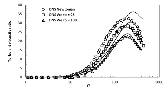
Figure 12 Comparison between the predictions of the turbulent viscosity ratio by the present model predictions and DNS data of13 for turbulent channel flow with R e τ =395 MathType@MTEF@5@5@+= feaagKart1ev2aqatCvAUfeBSjuyZL2yd9gzLbvyNv2CaerbuLwBLn hiov2DGi1BTfMBaeXatLxBI9gBaerbd9wDYLwzYbItLDharqqtubsr 4rNCHbGeaGqiVu0Je9sqqrpepC0xbbL8F4rqqrFfpeea0xe9Lq=Jc9 vqaqpepm0xbba9pwe9Q8fs0=yqaqpepae9pg0FirpepeKkFr0xfr=x fr=xb9adbaqaaeGaciGaaiaabeqaamaabaabaaGcbaqcLbsaqaaaaa aaaaWdbiaadkfacaWGLbqcfa4damaaBaaaleaajugWa8qacqaHepaD aSWdaeqaaKqzGeWdbiabg2da9iaaiodacaaI5aGaaGynaaaa@4031@ , L=30 MathType@MTEF@5@5@+= feaagKart1ev2aqatCvAUfeBSjuyZL2yd9gzLbvyNv2CaerbuLwBLn hiov2DGi1BTfMBaeXatLxBI9gBaerbd9wDYLwzYbItLDharqqtubsr 4rNCHbGeaGqiVu0Je9sqqrpepC0xbbL8F4rqqrFfpeea0xe9Lq=Jc9 vqaqpepm0xbba9pwe9Q8fs0=yqaqpepae9pg0FirpepeKkFr0xfr=x fr=xb9adbaqaaeGaciGaaiaabeqaamaabaabaaGcbaqcLbsaqaaaaa aaaaWdbiaadYeacqGH9aqpcaaIZaGaaGimaaaa@39F4@ and β=0.9 MathType@MTEF@5@5@+= feaagKart1ev2aaatCvAUfeBSjuyZL2yd9gzLbvyNv2CaerbuLwBLn hiov2DGi1BTfMBaeXatLxBI9gBaerbd9wDYLwzYbItLDharqqtubsr 4rNCHbGeaGqiVu0Je9sqqrpepC0xbbL8F4rqqrFfpeea0xe9Lq=Jc9 vqaqpepm0xbba9pwe9Q8fs0=yqaqpepae9pg0FirpepeKkFr0xfr=x fr=xb9adbaqaaeGaciGaaiaabeqaamaabaabaaGcbaqcLbsaqaaaaa aaaaWdbiabek7aIjabg2da9iaaicdacaGGUaGaaGyoaaaa@3B7B@ at W e τo =25 MathType@MTEF@5@5@+= feaagKart1ev2aaatCvAUfeBSjuyZL2yd9gzLbvyNv2CaerbuLwBLn hiov2DGi1BTfMBaeXatLxBI9gBaerbd9wDYLwzYbItLDharqqtubsr 4rNCHbGeaGqiVu0Je9sqqrpepC0xbbL8F4rqqrFfpeea0xe9Lq=Jc9 vqaqpepm0xbba9pwe9Q8fs0=yqaqpepae9pg0FirpepeKkFr0xfr=x fr=xb9adbaqaaeGaciGaaiaabeqaamaabaabaaGcbaqcLbsaqaaaaa aaaaWdbiaadEfacaWGLbqcfa4damaaBaaaleaajugWa8qacqaHepaD caWGVbaal8aabeaajugib8qacqGH9aqpcaaIYaGaaGynaaaa@4065@ and W e τo =100 MathType@MTEF@5@5@+= feaagKart1ev2aaatCvAUfeBSjuyZL2yd9gzLbvyNv2CaerbuLwBLn hiov2DGi1BTfMBaeXatLxBI9gBaerbd9wDYLwzYbItLDharqqtubsr 4rNCHbGeaGqiVu0Je9sqqrpepC0xbbL8F4rqqrFfpeea0xe9Lq=Jc9 vqaqpepm0xbba9pwe9Q8fs0=yqaqpepae9pg0FirpepeKkFr0xfr=x fr=xb9adbaqaaeGaciGaaiaabeqaamaabaabaaGcbaqcLbsaqaaaaa aaaaWdbiaadEfacaWGLbWcpaWaaSbaaeaajugWa8qacqaHepaDcaWG Vbaal8aabeaajugib8qacqGH9aqpcaaIXaGaaGimaiaaicdaaaa@408B@ .

Figure 13 Comparison between the predictions of the turbulent viscosity ratio by the present model predictions and both DNS model and RANS model of25 for turbulent channel flow with R e τ =395 MathType@MTEF@5@5@+= feaagKart1ev2aqatCvAUfeBSjuyZL2yd9gzLbvyNv2CaerbuLwBLn hiov2DGi1BTfMBaeXatLxBI9gBaerbd9wDYLwzYbItLDharqqtubsr 4rNCHbGeaGqiVu0Je9sqqrpepC0xbbL8F4rqqrFfpeea0xe9Lq=Jc9 vqaqpepm0xbba9pwe9Q8fs0=yqaqpepae9pg0FirpepeKkFr0xfr=x fr=xb9adbaqaaeGaciGaaiaabeqaamaabaabaaGcbaqcLbsaqaaaaa aaaaWdbiaadkfacaWGLbqcfa4damaaBaaaleaajugWa8qacqaHepaD aSWdaeqaaKqzGeWdbiabg2da9iaaiodacaaI5aGaaGynaaaa@4031@ , L=30 MathType@MTEF@5@5@+= feaagKart1ev2aqatCvAUfeBSjuyZL2yd9gzLbvyNv2CaerbuLwBLn hiov2DGi1BTfMBaeXatLxBI9gBaerbd9wDYLwzYbItLDharqqtubsr 4rNCHbGeaGqiVu0Je9sqqrpepC0xbbL8F4rqqrFfpeea0xe9Lq=Jc9 vqaqpepm0xbba9pwe9Q8fs0=yqaqpepae9pg0FirpepeKkFr0xfr=x fr=xb9adbaqaaeGaciGaaiaabeqaamaabaabaaGcbaqcLbsaqaaaaa aaaaWdbiaadYeacqGH9aqpcaaIZaGaaGimaaaa@39F4@ and β=0.9 MathType@MTEF@5@5@+= feaagKart1ev2aaatCvAUfeBSjuyZL2yd9gzLbvyNv2CaerbuLwBLn hiov2DGi1BTfMBaeXatLxBI9gBaerbd9wDYLwzYbItLDharqqtubsr 4rNCHbGeaGqiVu0Je9sqqrpepC0xbbL8F4rqqrFfpeea0xe9Lq=Jc9 vqaqpepm0xbba9pwe9Q8fs0=yqaqpepae9pg0FirpepeKkFr0xfr=x fr=xb9adbaqaaeGaciGaaiaabeqaamaabaabaaGcbaqcLbsaqaaaaa aaaaWdbiabek7aIjabg2da9iaaicdacaGGUaGaaGyoaaaa@3B7B@ at W e τo =25 MathType@MTEF@5@5@+= feaagKart1ev2aaatCvAUfeBSjuyZL2yd9gzLbvyNv2CaerbuLwBLn hiov2DGi1BTfMBaeXatLxBI9gBaerbd9wDYLwzYbItLDharqqtubsr 4rNCHbGeaGqiVu0Je9sqqrpepC0xbbL8F4rqqrFfpeea0xe9Lq=Jc9 vqaqpepm0xbba9pwe9Q8fs0=yqaqpepae9pg0FirpepeKkFr0xfr=x fr=xb9adbaqaaeGaciGaaiaabeqaamaabaabaaGcbaqcLbsaqaaaaa aaaaWdbiaadEfacaWGLbqcfa4damaaBaaaleaajugWa8qacqaHepaD caWGVbaal8aabeaajugib8qacqGH9aqpcaaIYaGaaGynaaaa@4065@ and W e τo =100 MathType@MTEF@5@5@+= feaagKart1ev2aaatCvAUfeBSjuyZL2yd9gzLbvyNv2CaerbuLwBLn hiov2DGi1BTfMBaeXatLxBI9gBaerbd9wDYLwzYbItLDharqqtubsr 4rNCHbGeaGqiVu0Je9sqqrpepC0xbbL8F4rqqrFfpeea0xe9Lq=Jc9 vqaqpepm0xbba9pwe9Q8fs0=yqaqpepae9pg0FirpepeKkFr0xfr=x fr=xb9adbaqaaeGaciGaaiaabeqaamaabaabaaGcbaqcLbsaqaaaaa aaaaWdbiaadEfacaWGLbWcpaWaaSbaaeaajugWa8qacqaHepaDcaWG Vbaal8aabeaajugib8qacqGH9aqpcaaIXaGaaGimaiaaicdaaaa@408B@ .

Test the present model against experimental results

The present model was tested against the experimental data of Warholic M et al30 at different values of the polymer concentration. The channel used in the experiments was with a height of 5.08 cm and 3 m length. The master polymer was a solution of Percol-727, which is a copolymer of polyacrylamide and sodium acrylamide. The simulations were performed at the same dimensions and frictional Reynolds number ( R e τ =778.4 ) MathType@MTEF@5@5@+= feaagKart1ev2aaatCvAUfeBSjuyZL2yd9gzLbvyNv2CaerbuLwBLn hiov2DGi1BTfMBaeXatLxBI9gBaerbd9wDYLwzYbItLDharqqtubsr 4rNCHbGeaGqiVu0Je9sqqrpepC0xbbL8F4rqqrFfpeea0xe9Lq=Jc9 vqaqpepm0xbba9pwe9Q8fs0=yqaqpepae9pg0FirpepeKkFr0xfr=x fr=xb9adbaqaaeGaciGaaiaabeqaamaabaabaaGcbaqcfaieaaaaaa aaa8qadaqadaGcpaqaaKqzGeWdbiaadkfacaWGLbqcfa4damaaBaaa leaajugWa8qacqaHepaDaSWdaeqaaKqzGeWdbiabg2da9iaaiEdaca aI3aGaaGioaiaac6cacaaI0aaakiaawIcacaGLPaaaaaa@43EF@ . The polymer parameters for the simulations were calculated by32 based on33 experimental results. The mean velocity profile and  were computed and compared with the experimental results at the three regions of drag reduction (i.e. low, intermediate and high regions). Figure 14 shows a good prediction of the mean velocity profile and the positive shift of the buffer layer with DR, which is well captured in low and intermediate drag reduction regions. At high drag reduction region, the deviation between predicted numerical and experimental mean velocity profile is very large and increased with increasing . Table 2 shows the predicted  variation with the polymer concentration changes in three regions. Also, the relative error with the experimental results is listed in Table 2.
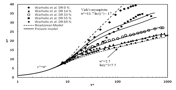
Figure 14 Comparison between the predicted mean velocity by the present model and the experimental data of.30

Concentration (ppm)

W e τo MathType@MTEF@5@5@+= feaagKart1ev2aqatCvAUfeBSjuyZL2yd9gzLbvyNv2CaerbuLwBLn hiov2DGi1BTfMBaeXatLxBI9gBaerbd9wDYLwzYbItLDharqqtubsr 4rNCHbGeaGqiVu0Je9sqqrpepC0xbbL8F4rqqrFfpeea0xe9Lq=Jc9 vqaqpepm0xbba9pwe9Q8fs0=yqaqpepae9pg0FirpepeKkFr0xfr=x fr=xb9adbaqaaeGaciGaaiaabeqaamaabaabaaGcbaqcLbsaqaaaaa aaaaWdbiaadEfacaWGLbWcpaWaaSbaaeaajugWa8qacqaHepaDcaWG Vbaal8aabeaaaaa@3CB8@

Experimental DR

Model DR

Relative error %

0.24

16.5

14

13.1

6.4

1.25

36.5

33

34.6

4.8

3

74

55

50.5

7.5

50

100

69

59.7

13.5

Table 2 Comparison between the drag reduction predicted by the present model and the experimental data of Warholic M et al.30

Conclusions

In the present study, the standard kω MathType@MTEF@5@5@+= feaagKart1ev2aaatCvAUfeBSjuyZL2yd9gzLbvyNv2CaerbuLwBLn hiov2DGi1BTfMBaeXatLxBI9gBaerbd9wDYLwzYbItLDharqqtubsr 4rNCHbGeaGqiVu0Je9sqqrpepC0xbbL8F4rqqrFfpeea0xe9Lq=Jc9 vqaqpepm0xbba9pwe9Q8fs0=yqaqpepae9pg0FirpepeKkFr0xfr=x fr=xb9adbaqaaeGaciGaaiaabeqaamaabaabaaGcbaqcLbsaqaaaaa aaaaWdbiaadUgacqGHsislcqaHjpWDaaa@3A4F@ eddy viscosity turbulence model has been investigated for the turbulent drag reducing fluid flow. This model has been developed to predict the drag reduction and the mean velocity profile in low and intermediate regions without using any additional constitutive equations. Moreover, an expression for a new average eddy viscosity equation, which is directly related to the fluid and flow rheological parameters, has been developed. In the present model, the trace of the conformation tensor in FENE-P eddy viscosity models was replaced with a new M we MathType@MTEF@5@5@+= feaagKart1ev2aaatCvAUfeBSjuyZL2yd9gzLbvyNv2CaerbuLwBLn hiov2DGi1BTfMBaeXatLxBI9gBaerbd9wDYLwzYbItLDharqqtubsr 4rNCHbGeaGqiVu0Je9sqqrpepC0xbbL8F4rqqrFfpeea0xe9Lq=Jc9 vqaqpepm0xbba9pwe9Q8fs0=yqaqpepae9pg0FirpepeKkFr0xfr=x fr=xb9adbaqaaeGaciGaaiaabeqaamaabaabaaGcbaqcLbsaqaaaaa aaaaWdbiaad2eal8aadaWgaaqaaKqzadWdbiaadEhacaWGLbaal8aa beaaaaa@3AF0@ function. This function involves the polymer parameters which affect in the value of the drag reduction. The DNS results were used to predict the M we MathType@MTEF@5@5@+= feaagKart1ev2aaatCvAUfeBSjuyZL2yd9gzLbvyNv2CaerbuLwBLn hiov2DGi1BTfMBaeXatLxBI9gBaerbd9wDYLwzYbItLDharqqtubsr 4rNCHbGeaGqiVu0Je9sqqrpepC0xbbL8F4rqqrFfpeea0xe9Lq=Jc9 vqaqpepm0xbba9pwe9Q8fs0=yqaqpepae9pg0FirpepeKkFr0xfr=x fr=xb9adbaqaaeGaciGaaiaabeqaamaabaabaaGcbaqcLbsaqaaaaa aaaaWdbiaad2eal8aadaWgaaqaaKqzadWdbiaadEhacaWGLbaal8aa beaaaaa@3AF0@ function using ANSYS-fluent 16.1 software. A UDF code was interpreted to ANSYS-Fluent 16.1 solver and the Newtonian eddy viscosity was replaced with a new average eddy viscosity equation. The developed model was initially validated with the DNS data and the results of different RANS turbulence models for different values of the frictional Reynolds number and polymer parameters. Also, the developed model was validated by the experimental results at the same flow conditions in low, intermediate and high drag reduction regions. The results obtained from this study can be summarized as follows:

  1. Good agreements between the model predictions and both of the DNS and the experimental results are obtained in low and intermediate drag reduction regions (DR<60%) MathType@MTEF@5@5@+= feaagKart1ev2aaatCvAUfeBSjuyZL2yd9gzLbvyNv2CaerbuLwBLn hiov2DGi1BTfMBaeXatLxBI9gBaerbd9wDYLwzYbItLDharqqtubsr 4rNCHbGeaGqiVu0Je9sqqrpepC0xbbL8F4rqqrFfpeea0xe9Lq=Jc9 vqaqpepm0xbba9pwe9Q8fs0=yqaqpepae9pg0FirpepeKkFr0xfr=x fr=xb9adbaqaaeGaciGaaiaabeqaamaabaabaaGcbaqcLbsacaGGOa GaamiraiaadkfacqGH8aapcaaI2aGaaGimaiaacwcacaGGPaaaaa@3CA5@ .
  2. The predicted turbulent viscosity ratio agrees well with the DNS results at low and intermediate drag reduction regions.
  3. The developed model is an extension of the standard RANS kω model Consequently, the model could be used at higher values of Reynolds number and complex geometries, which becomes more practical than the DNS model.
  4. The model is simulated without any additional constitutive equations. So, the model reduces the running time and the cost of simulation.
  5. The model also can be used to predict the DR and the mean velocity profile in the developing zone, which may contain heterogeneous polymer solutions.

Acknowledgments

None.

Conflicts of interest

The author declares that there is no conflict of interest.

References

  1. Abubakar A, Al Wahaibi T, Al Wahaibi Y, et al. Roles of drag reducing polymers in single‒and multi‒phase flows. Chemical Engineering Research and Design. 2014;92(11):2153‒2181.
  2. Toms B. Proc. 1st Intern. Congr on Rheology. p. II‒IB. Amsterdam: North‒Holland Publ; 1948.
  3. Virk PS. Drag reduction fundamentals. AIChE Journal. 1975;21(4):625‒656.
  4. Mizushina T, Usui H, Toshiba T. Turbulent pipe flow of dilute polymer solutions. Journal of Chemical Engineering of Japan. 1974;7(3):162‒167.
  5. Durst F, Rastogi A. Calculations of turbulent boundary layer flows with drag reducing polymer additives. The Physics of Fluids. 1977;20(12):1975‒1985.
  6. Malin M. Turbulent pipe flow of power‒law fluids. International communications in heat and mass transfer. 1997;24(7):977‒988.
  7. Cruz D, Pinho F. Turbulent pipe flow predictions with a low Reynolds number k–ε model for drag reducing fluids. Journal of Non‒Newtonian Fluid Mechanics. 2003;114(2):109‒148.
  8. Pinho F. A GNF framework for turbulent flow models of drag reducing fluids and proposal for a k–ε type closure. Journal of Non‒Newtonian Fluid Mechanics. 2003;114(2):149‒184.
  9. Resende P, Escudier M, Presti F, et al. Numerical predictions and measurements of Reynolds normal stresses in turbulent pipe flow of polymers. International Journal of Heat and Fluid Flow. 2006;27(2):204‒219.
  10. Ptasinski PB, Boersma F, Nieuwstadt M, et al. Turbulent channel flow near maximum drag reduction: simulations, experiments and mechanisms. Journal of Fluid Mechanics. 2003;490:251‒291.
  11. Sureshkumar R, Beris AN, Handler RA. Direct numerical simulation of the turbulent channel flow of a polymer solution. Physics of Fluids. 1997;9(3):743‒755.
  12. De Angelis E, Casciola C, Piva R. DNS of wall turbulence: dilute polymers and self‒sustaining mechanisms. Computers & fluids. 2002;31(4):495‒507.
  13. Li C, Gupta V, Sureshkumar R, et al. Turbulent channel flow of dilute polymeric solutions: drag reduction scaling and an eddy viscosity model. Journal of Non‒Newtonian Fluid Mechanics. 2006;139(3):177‒189.
  14. Dimitropoulos CD, Sureshkumar R, Beris AN. Direct numerical simulation of viscoelastic turbulent channel flow exhibiting drag reduction: effect of the variation of rheological parameters. Journal of Non‒Newtonian Fluid Mechanics. 1998;79(2):433‒468.
  15. Housiadas KD, Beris AN. An efficient fully implicit spectral scheme for DNS of turbulent viscoelastic channel flow. Journal of Non‒Newtonian Fluid Mechanics. 2004;122(1):243‒262.
  16. Dimitropoulos CD, Sureshkumar R, Beris AN, et al. Budgets of Reynolds stress, kinetic energy and streamwise enstrophy in viscoelastic turbulent channel flow. Physics of Fluids. 2001;13(4):1016‒1027.
  17. Li CF, Sureshkumar R, Khomami B. Influence of rheological parameters on polymer induced turbulent drag reduction. Journal of Non‒Newtonian Fluid Mechanics. 2006;140(1):23‒40.
  18. Housiadas KD, Beris AN, Handler RA. Viscoelastic effects on higher order statistics and on coherent structures in turbulent channel flow. Physics of Fluids. 2005;17(3).
  19. Kimm K, Li CF, Sureshkumar R, et al. Effects of polymer stresses on eddy structures in drag‒reduced turbulent channel flow. Journal of Fluid Mechanics. 2007;584:281‒299.
  20. Pinho FT, Li CF, Younis BA, et al. A low Reynolds number turbulence closure for viscoelastic fluids. Journal of Non‒Newtonian Fluid Mechanics. 2008;154(2):89‒108.
  21. Nagano Y, Hishida M. Improved form of the k‒ε model for wall turbulent shear flows. Journal of Fluids Engineering. 1987;109(2):156‒160.
  22. Iaccarino G, Shaqfeh ES, Dubief Y. Reynolds‒averaged modeling of polymer drag reduction in turbulent flows. Journal of Non‒Newtonian Fluid Mechanics. 2010;165(7):376‒384.
  23. Durbin P. Separated Flow Computations with the k‒ ‒v^ 2 Model. AIAA journal. 1995;33(4).
  24. Resende P, Kim K, Younis B, et al. A FENE‒P k–ε turbulence model for low and intermediate regimes of polymer‒induced drag reduction. Journal of Non‒Newtonian Fluid Mechanics. 2011;166(12):639‒660.
  25. Resende P, Pinho F, Younis B, et al. Development of a Low‒Reynolds‒number k‒ω Model for FENE‒P Fluids. Flow, turbulence and combustion. 2013;90(1):69‒94.
  26. Wilcox DC. Turbulence modeling for CFD, DCW Industries Inc, Canada; 1998.
  27. Masoudian M, Kim K, Pinho FT, et al. A viscoelastic k‒ε‒v2¯‒f turbulent flow model valid up to the maximum drag reduction limit. Journal of Non‒Newtonian Fluid Mechanics. 2013;202:99‒111.
  28. Masoudian M, Pinho FT, Kim K. A RANS model for heat transfer reduction in viscoelastic turbulent flow. International Journal of Heat and Mass Transfer. 2016;100:332‒346.
  29. Azad S, Riasi A, Moghadam HA. Parametric study of a viscoelastic RANS turbulence model in the fully developed channel flow. Journal of Computational Applied Mechanics. 2017:48(1):65‒74.
  30. Warholic M, Massah H, Hanratty T. Influence of drag‒reducing polymers on turbulence: effects of Reynolds number, concentration and mixing. Experiments in fluids. 1999;27(5):461‒472.
  31. Housiadas KD, Beris AN. Polymer‒induced drag reduction: Effects of the variations in elasticity and inertia in turbulent viscoelastic channel flow. Physics of Fluids. 2003;15(8):2369‒2384.
  32. Lee DH. Skin‒Friction Drag Reduction by Dilute Polymer Solutions in Turbulent Channel Flow. The University of Michigan. 2010.
  33. Cruz D, Pinho F, Resende P. Modelling the new stress for improved drag reduction predictions of viscoelastic pipe flow. Journal of Non‒Newtonian Fluid Mechanics. 2004;121(2):127‒141.
Creative Commons Attribution License

©2018 Rabie, et al. This is an open access article distributed under the terms of the, which permits unrestricted use, distribution, and build upon your work non-commercially.