In this paper, I have presented an analytical solution to the problem of plane Poiseuille flow in a channel filled with a porous medium. Nield et al.,¹ have expressed it in terms of elliptic integrals. I express it in an equivalent, but a more conventional form, in terms of Weierstrass elliptic function. I also present the R code to plot the velocity profile and compute the flux.

The flow of an incompressible, Newtonian fluid through a porous medium of porosity $\epsilon$  and permeability $K$  is described by the equation²
$\frac{\partial \overrightarrow{u}}{\partial t}+\overrightarrow{u}\mathrm{.}\nabla \left(\frac{\overrightarrow{u}}{\epsilon }\right)\mathrm{<mo>=</mo>}-\nabla \left(\frac{p\epsilon }{\rho }\right)+{\nu }_e\Delta \overrightarrow{u}+\overrightarrow{F}\mathrm{,}$                                           (1)
where$\rho$ is the density of the fluid, $\overrightarrow{u}$  is the velocity,$p$  the pressure,${\nu }_e$  the effective viscosity,$\nu$  the kinematic viscosity, $\Delta$ denotes the Laplace operator and the total force is
$\overrightarrow{F}\mathrm{<mo>=</mo>}{\overrightarrow{F}}_b-\frac{\epsilon \nu }{K}\overrightarrow{u}-\frac{\epsilon F_0}{\sqrt{K}}u\overrightarrow{u}\mathrm{.}$                                                                 (2)
It is a sum of the body force ${\overrightarrow{F}}_b$  and the effect of the porosity of the medium. The geometric function$F_0$ in equation (2) depends only on the porosity and the nature of the solid particle matrix of the porous medium. For a fully developed and steady flow, the left hand side of equation (1) vanishes. Further, if the flow is driven only by a constant pressure gradient and not an external body force, then equation (1) becomes
${\nu }_e\Delta \overrightarrow{u}-\frac{\epsilon \nu }{K}\overrightarrow{u}-\frac{\epsilon F_0}{\sqrt{K}}u\overrightarrow{u}+\epsilon \overrightarrow{G}\mathrm{<mo>=</mo>0,}$                                                     (3)
where $\rho \overrightarrow{G}\mathrm{<mo>=</mo>}-\nabla p$ . I will solve equation (3) for a flow between parallel solid plates with a porous medium between them.

Consider a steady, fully-developed flow of a fluid along the $x$  axis between two infinite parallel plates, a distance $H$ apart. Let the plates concide with planes $y\mathrm{<mo>=</mo>0}$  and $y\mathrm{<mo>=</mo>}H$ . If the channel is long enough that the end effects are negligible along most of the channel's length then we can express the fluid's velocity along the $x$  axis as $u\mathrm{<mo\; stretchy="false">(</mo>}y\mathrm{<mo\; stretchy="false">)</mo>}$ . Equation (3), in this case, becomes
$\frac{{\nu }_e}{\epsilon }{u}^{\text{'}\text{'}}-\frac{\nu }{K}u-\frac{F_0}{\sqrt{K}}{u}^2+\epsilon G\mathrm{<mo>=</mo>0,}$                                                      (4)
where $u^{\text{'}\text{'}}$  denotes the second derivative with respect to $y$ . Since the channel is bounded by solid walls, the usual no-slip boundary conditions apply. I will solve (4) subject to the conditions $u\mathrm{<mo\; stretchy="false">(</mo>}y\mathrm{<mo>=</mo>0<mo\; stretchy="false">)</mo><mo>=</mo>0}$  and $u^{\text{'}}\mathrm{<mo\; stretchy="false">(</mo>}H\mathrm{<mo>/</mo>2<mo\; stretchy="false">)</mo><mo>=</mo>0}$ , that is, the velocity has an extremum (actually, a maximum) at the center of the channel. Nield et al.,¹ have given an analytical solution which expresses the coordinate $y$  as an elliptic integral in the velocity $u$ . I will develop an equivalent solution in which $u$  is expressed as a Weierstrass elliptic function of $y.$

 We convert equation (4) in a non-dimensional form using the relations,
$u_{\star }\mathrm{<mo>=</mo>}\frac{u}{U}$                                                                                            (5)
$y_{\star }\mathrm{<mo>=</mo>}\frac{y}{H}$                                                                                           (6)
$G_{\star }\mathrm{<mo>=</mo>}\frac{HG}{U^2}\mathrm{,}$                                                                                       (7)
where $U$  is the velocity at the center of the channel, and the dimensionless quantities
$Re\mathrm{<mo>=</mo>}\frac{HU}{\nu }$                                                                                        (8)
$Da\mathrm{<mo>=</mo>}\frac{K}{H^2}$                                                                                        (9)
$J\mathrm{<mo>=</mo>}\frac{{\nu }_e}{\nu }\mathrm{.}$                                                                                           (10)
$Re$ , $Da$  and $J$  are the Reynold's number, the Darcy number and the viscosity ratio of the flow. Dropping the $\star$  subscript for sake of notation clarity, we get,
$u^{\text{'}\text{'}}-A^2{u}^2-B^{2}u+C^2\mathrm{<mo>=</mo>0,}$                                                             (11)
where
$A^2\mathrm{<mo>=</mo>}\frac{F_0\epsilon Re}{J\sqrt{Da}}$                                                                                  (12)
$B^2\mathrm{<mo>=</mo>}\frac{\epsilon }{JDa}$                                                                                      (13)
$C^2\mathrm{<mo>=</mo>}\frac{{\epsilon }^{2}ReG}{J}$                                                                                  (14)
are all positive numbers. Introduce a new variable $u_1\mathrm{<mo\; stretchy="false">(</mo>}y\mathrm{<mo\; stretchy="false">)</mo>}$ ,
$u_1\mathrm{<mo\; stretchy="false">(</mo>}y\mathrm{<mo\; stretchy="false">)</mo><mo>=</mo>}Au\mathrm{<mo\; stretchy="false">(</mo>}y\mathrm{<mo\; stretchy="false">)</mo>}+\frac{1}{2}\frac{B^2}{A}\mathrm{,}$                                                                   (15)
so that equation (11) becomes,
$u_1^{\text{'}\text{'}}-A{u}_1^2+\left(A{C}^2+\frac{B^4}{4A}\right)\mathrm{<mo>=</mo>0,}$                                                         (16)
Multiplying equation (16) by $u_1^{\text{'}}$ , the first derivative of $u_1\mathrm{<mo\; stretchy="false">(</mo>}y\mathrm{<mo\; stretchy="false">)</mo>}$ with respect to $y$ , and integrating we get,
${\left(u_1^{\text{'}}\right)}^2-\frac{2}{3}A{u}_1^3+2\left(A{C}^2+\frac{B^4}{4A}\right)u_1+\frac{36g_3}{A^2}\mathrm{<mo>=</mo>0,}$                               (17)
where $36g_3\mathrm{<mo>/</mo>}{A}^2$  is a constant of integration. Introduce yet another variable, $u_2\mathrm{<mo\; stretchy="false">(</mo>}y\mathrm{<mo\; stretchy="false">)</mo><mo>=</mo><mo\; stretchy="false">(</mo>}A\mathrm{<mo>/</mo>6<mo\; stretchy="false">)</mo>}{u}_1\mathrm{<mo\; stretchy="false">(</mo>}y\mathrm{<mo\; stretchy="false">)</mo>}$ , to transform equation (17) to
${\left(u_2^{\text{'}}\right)}^2\mathrm{<mo>=</mo>4}{u}_2^3-\frac{1}{3}\left(A^2{C}^2+\frac{B^4}{4}\right)u_2-g_3\mathrm{.}$                                           (18)
This equation is of the form,
${\mathrm{<mo\; stretchy="false">(</mo>}{u}_2^{\text{'}}\mathrm{<mo\; stretchy="false">)</mo>}}^2\mathrm{<mo>=</mo>4}{u}_2^3-g_2{u}_2-g_3\mathrm{,}$                                                                (19)
where
$g_2\mathrm{<mo>=</mo>}\frac{1}{3}\left(A^2{C}^2+\frac{B^4}{4}\right)$                                                                     (20)
Its solution is $u_2\mathrm{<mo\; stretchy="false">(</mo>}y\mathrm{<mo\; stretchy="false">)</mo><mo>=</mo>}\wp \mathrm{<mo\; stretchy="false">(</mo>}y+k_1\mathrm{<mo>;</mo>}{g}_2\mathrm{,}{g}_3\mathrm{<mo\; stretchy="false">)</mo>}$ , where $k_1$  is another constant of integration. The function $\wp$  is the Weierstrass elliptic function with invariants $g_2$  and $g_3$ .³ Therefore, the solution of (11) is
$u\mathrm{<mo\; stretchy="false">(</mo>}y\mathrm{<mo\; stretchy="false">)</mo><mo>=</mo>}\frac{6}{A^2}\left[\wp \left(y+k_1\mathrm{<mo>|</mo>}\frac{1}{3}\left(A^2{C}^2+\frac{B^4}{4}\right)\mathrm{,}{g}_3\right)-\frac{B^2}{12}\right]$                        (21)
The constants $g_3$ and $k_1$  are found using the boundary conditions.

Some properties of Weierstrass elliptic function

The Weierstrass elliptic function is defined as the solution of the differential equation,
${\left[{\wp }^{\text{'}}\mathrm{<mo\; stretchy="false">(</mo>}u\mathrm{<mo\; stretchy="false">)</mo>}\right]}^2\mathrm{<mo>=</mo>4}{\wp }^3\mathrm{<mo\; stretchy="false">(</mo>}u\mathrm{<mo\; stretchy="false">)</mo>}-g_2\wp \mathrm{<mo\; stretchy="false">(</mo>}u\mathrm{<mo\; stretchy="false">)</mo>}-g_3\mathrm{,}$  (22)
where $u$  is a complex variable and $g_2$  and $g_3$ are complex constants, called invariants of $\wp$ . Weierstrass elliptic function is a doubly periodic function. We follow Lawden⁴ and call the periods $2{\omega }_1$  and $2{\omega }_3$ . There is another half period $2{\omega }_2$ , where ${\omega }_2\mathrm{<mo>=</mo>}-{\omega }_1-{\omega }_3$ . Whittaker et al.,³ denote the fundamental periods by ${\omega }_1$  and ${\omega }_2$  and define ${\omega }_3\mathrm{<mo>=</mo>}-{\omega }_1-{\omega }_2$ .) If the constants $e_j$ are defined as
$e_j\mathrm{<mo>=</mo>}\wp \mathrm{<mo\; stretchy="false">(</mo>}{\omega }_j\mathrm{<mo\; stretchy="false">)</mo>}$                                                                                     (23)
then it can be shown that [by Lawden⁴ p.160] they are solutions of the cubic equation $4s^3-g_{2}s-g_3\mathrm{<mo>=</mo>0}$ . Further, they are related to the invariants as
$g_2\mathrm{<mo>=</mo>}-\mathrm{4<mo\; stretchy="false">(</mo>}{e}_1{e}_2+e_2{e}_3+e_3{e}_1\mathrm{<mo\; stretchy="false">)</mo>}$                                                             (24)
$g_3\mathrm{<mo>=</mo>4}{e}_1{e}_2{e}_3$                                                                                   (25)
Additionally [Lawden⁴ p.159],
$e_1+e_2+e_3\mathrm{<mo>=</mo>0}$                                                                               (26)

The discriminant of the cubic equation $4t^3-g_{2}t-g_3\mathrm{<mo>=</mo>0}$  is $D\mathrm{<mo>=</mo>16<mo\; stretchy="false">(</mo>}{g}_2^3-27g_3^2\mathrm{<mo\; stretchy="false">)</mo>}$ .
If

1. $D\mathrm{<mo>></mo>0}$ , then all roots of $4t^3-g_{2}t-g_3\mathrm{<mo>=</mo>0}$  are real and distinct.
2. $D\mathrm{<mo>=</mo>0}$ , then the roots of $4t^3-g_{2}t-g_3\mathrm{<mo>=</mo>0}$  are real and not distinct.
3. $D\mathrm{<mo><</mo>0}$ , then $4t^3-g_{2}t-g_3\mathrm{<mo>=</mo>0}$  has one real root and two complex roots. The complex roots are conjugates of each other.

Theorem 1: If the invariants of Weierstrass elliptic function $\wp$  are real and if the roots of the cubic $4s^3-g_{2}s-g_3\mathrm{<mo>=</mo>0}$  are real then ${\omega }_1$  is real and ${\omega }_3$  is imaginary.

Proof: The constants $e_1\mathrm{,}{e}_2\mathrm{,}{e}_3$  are solutions of the cubic $4s^3-g_{2}s-g_3\mathrm{<mo>=</mo>0}$ . If they are all real, we can choose them to be such that $e_1\mathrm{<mo>></mo>}{e}_2\mathrm{<mo>></mo>}{e}_3$ . Then (22) can be written as
${\left\{\mathrm{<mo\; stretchy="false">(</mo>}\wp \mathrm{<mo\; stretchy="false">(</mo>}u\mathrm{<mo\; stretchy="false">)</mo>}-e_1\mathrm{<mo\; stretchy="false">)</mo><mo\; stretchy="false">(</mo>}\wp \mathrm{<mo\; stretchy="false">(</mo>}u\mathrm{<mo\; stretchy="false">)</mo>}-e_2\mathrm{<mo\; stretchy="false">)</mo><mo\; stretchy="false">(</mo>}\wp \mathrm{<mo\; stretchy="false">(</mo>}u\mathrm{<mo\; stretchy="false">)</mo>}-e_3\mathrm{<mo\; stretchy="false">)</mo>}\right\}}^{\mathrm{1<mo>/</mo>2}}\mathrm{<mo>=</mo>}-\frac{1}{2}{\wp }^{\text{'}}\mathrm{<mo\; stretchy="false">(</mo>}u\mathrm{<mo\; stretchy="false">)</mo>}$
that is,
$\frac{d\wp \mathrm{<mo\; stretchy="false">(</mo>}u\mathrm{<mo\; stretchy="false">)</mo>}}{\sqrt{\mathrm{4<mo\; stretchy="false">(</mo>}\wp \mathrm{<mo\; stretchy="false">(</mo>}u\mathrm{<mo\; stretchy="false">)</mo>}-e_1\mathrm{<mo\; stretchy="false">)</mo><mo\; stretchy="false">(</mo>}\wp \mathrm{<mo\; stretchy="false">(</mo>}u\mathrm{<mo\; stretchy="false">)</mo>}-e_2\mathrm{<mo\; stretchy="false">)</mo><mo\; stretchy="false">(</mo>}\wp \mathrm{<mo\; stretchy="false">(</mo>}u\mathrm{<mo\; stretchy="false">)</mo>}-e_3\mathrm{<mo\; stretchy="false">)</mo>}}}\mathrm{<mo>=</mo>}-du$
equivalently,
$\frac{dt}{\sqrt{\mathrm{4<mo\; stretchy="false">(</mo>}t-e_1\mathrm{<mo\; stretchy="false">)</mo><mo\; stretchy="false">(</mo>}t-e_2\mathrm{<mo\; stretchy="false">)</mo><mo\; stretchy="false">(</mo>}t-e_3\mathrm{<mo\; stretchy="false">)</mo>}}}\mathrm{<mo>=</mo>}-du\mathrm{,}$
where $t\mathrm{<mo>=</mo>}\wp \mathrm{<mo\; stretchy="false">(</mo>}u\mathrm{<mo\; stretchy="false">)</mo>}$ . Integrating this equation so that $u$  goes from $0$ to $U$ , and hence $t$  goes from $\wp \mathrm{<mo\; stretchy="false">(</mo>0<mo\; stretchy="false">)</mo>}$  to $\wp \mathrm{<mo\; stretchy="false">(</mo>}U\mathrm{<mo\; stretchy="false">)</mo>}$ , we have two possibilities because of the double pole of $\wp$  at the origin,
${\displaystyle {\int }_{\infty }^{\wp \mathrm{<mo\; stretchy="false">(</mo>}U\mathrm{<mo\; stretchy="false">)</mo>}}}\frac{dt}{\sqrt{\mathrm{4<mo\; stretchy="false">(</mo>}t-e_1\mathrm{<mo\; stretchy="false">)</mo><mo\; stretchy="false">(</mo>}t-e_2\mathrm{<mo\; stretchy="false">)</mo><mo\; stretchy="false">(</mo>}t-e_3\mathrm{<mo\; stretchy="false">)</mo>}}}\mathrm{<mo>=</mo>}-U$                                              (27)
or
${\displaystyle {\int }_{-\infty }^{\wp \mathrm{<mo\; stretchy="false">(</mo>}U\mathrm{<mo\; stretchy="false">)</mo>}}}\frac{dt}{\sqrt{\mathrm{4<mo\; stretchy="false">(</mo>}t-e_1\mathrm{<mo\; stretchy="false">)</mo><mo\; stretchy="false">(</mo>}t-e_2\mathrm{<mo\; stretchy="false">)</mo><mo\; stretchy="false">(</mo>}t-e_3\mathrm{<mo\; stretchy="false">)</mo>}}}\mathrm{<mo>=</mo>}-U$                                              (28)

Choose $U\mathrm{<mo>=</mo>}{\omega }_1$  in equation (27), so that
${\omega }_1\mathrm{<mo>=</mo>}-{\displaystyle {\int }_{\infty }^{\wp \mathrm{<mo\; stretchy="false">(</mo>}{\omega }_1\mathrm{<mo\; stretchy="false">)</mo>}}}\frac{dt}{\sqrt{\mathrm{4<mo\; stretchy="false">(</mo>}t-e_1\mathrm{<mo\; stretchy="false">)</mo><mo\; stretchy="false">(</mo>}t-e_2\mathrm{<mo\; stretchy="false">)</mo><mo\; stretchy="false">(</mo>}t-e_3\mathrm{<mo\; stretchy="false">)</mo>}}}\mathrm{<mo>=</mo>}{\displaystyle {\int }_{e_1}^{\infty }}\frac{dt}{\sqrt{\mathrm{4<mo\; stretchy="false">(</mo>}t-e_1\mathrm{<mo\; stretchy="false">)</mo><mo\; stretchy="false">(</mo>}t-e_2\mathrm{<mo\; stretchy="false">)</mo><mo\; stretchy="false">(</mo>}t-e_3\mathrm{<mo\; stretchy="false">)</mo>}}}$
Since $e_1$  is the largest root of $\mathrm{4<mo\; stretchy="false">(</mo>}t-e_1\mathrm{<mo\; stretchy="false">)</mo><mo\; stretchy="false">(</mo>}t-e_2\mathrm{<mo\; stretchy="false">)</mo><mo\; stretchy="false">(</mo>}t-e_3\mathrm{<mo\; stretchy="false">)</mo><mo>=</mo>4}{t}^3-g_{2}t-g_3\mathrm{<mo>=</mo>0}$ , throughout the path of integration, the integrand stays finite. Further, the integrand is always real and hence ${\omega }_1$  is real.

Choose $U\mathrm{<mo>=</mo>}-{\omega }_3$  in equation (28), so that
${\omega }_3\mathrm{<mo>=</mo>}-{\displaystyle {\int }_{-\infty }^{\wp \mathrm{<mo\; stretchy="false">(</mo>}{\omega }_3\mathrm{<mo\; stretchy="false">)</mo>}}}\frac{dt}{\sqrt{\mathrm{4<mo\; stretchy="false">(</mo>}t-e_1\mathrm{<mo\; stretchy="false">)</mo><mo\; stretchy="false">(</mo>}t-e_2\mathrm{<mo\; stretchy="false">)</mo><mo\; stretchy="false">(</mo>}t-e_3\mathrm{<mo\; stretchy="false">)</mo>}}}\mathrm{<mo>=</mo>}-{\displaystyle {\int }_{-\infty }^{e_3}}\frac{dt}{\sqrt{\mathrm{4<mo\; stretchy="false">(</mo>}t-e_1\mathrm{<mo\; stretchy="false">)</mo><mo\; stretchy="false">(</mo>}t-e_2\mathrm{<mo\; stretchy="false">)</mo><mo\; stretchy="false">(</mo>}t-e_3\mathrm{<mo\; stretchy="false">)</mo>}}}$
or,
${\omega }_3\mathrm{<mo>=</mo>}i{\displaystyle {\int }_{-\infty }^{e_3}}\frac{dt}{\sqrt{\mathrm{4<mo\; stretchy="false">(</mo>}{e}_1-t\mathrm{<mo\; stretchy="false">)</mo><mo\; stretchy="false">(</mo>}{e}_2-t\mathrm{<mo\; stretchy="false">)</mo><mo\; stretchy="false">(</mo>}{e}_3-t\mathrm{<mo\; stretchy="false">)</mo>}}}$
Since $e_3$  is the smallest root of $\mathrm{4<mo\; stretchy="false">(</mo>}t-e_1\mathrm{<mo\; stretchy="false">)</mo><mo\; stretchy="false">(</mo>}t-e_2\mathrm{<mo\; stretchy="false">)</mo><mo\; stretchy="false">(</mo>}t-e_3\mathrm{<mo\; stretchy="false">)</mo><mo>=</mo>4}{t}^3-g_{2}t-g_3\mathrm{<mo>=</mo>0}$ , throughout the path of integration, the integrand stays finite. Further, the integrand is always real and hence ${\omega }_3$  is imaginary.

Remark: The converse of theorem 1 is also true [Lawden⁴ p.163]. That is, if ${\omega }_1$  is real and ${\omega }_3$  is imaginary then $e_j$ , the roots of $4s^3-g_{2}s-g_3\mathrm{<mo>=</mo>0}$  are all real.

If ${\omega }_1$  is real and ${\omega }_3$  is imaginary then section 6.11 shows that⁴
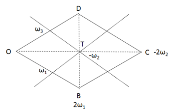
Theorem 2: $\wp$  takes real values on the the rectangle $OXAY$  in Figure 1, where $O\equiv \mathrm{<mo\; stretchy="false">(</mo>0,0<mo\; stretchy="false">)</mo>,}X\equiv \mathrm{<mo\; stretchy="false">(</mo>}{\omega }_1\mathrm{,0<mo\; stretchy="false">)</mo>,}A\equiv \mathrm{<mo\; stretchy="false">(</mo>}{\omega }_1\mathrm{,}{\omega }_3\mathrm{<mo\; stretchy="false">)</mo>}$  and $Y\equiv \mathrm{<mo\; stretchy="false">(</mo>0,}{\omega }_3\mathrm{<mo\; stretchy="false">)</mo>}$ . Further, if $u$  is taken round $OXAY$ , $\wp \mathrm{<mo\; stretchy="false">(</mo>}u\mathrm{<mo\; stretchy="false">)</mo>}$  decreases from $+\infty$  at $O$  to $e_1$  at $X$ , further decreases to $e_2$  along $XA$ , to $e_3$  along $AY$  and finally to $-\infty$  as it reaches the origin along $YA$ .

Figure 1 Positive discrimimant.

If the invariants $g_2$ and $g_3$  of the Weierstrass elliptic function are real but the discriminant of the cubic equation $4t^3-g_{2}t-g_3\mathrm{<mo>=</mo>0}$  is negative, then referring to Figure 2 or Handbook of Mathematical Functions with Formulas5, the function $\wp$  takes value $+\infty$  at $O$ . Its value decreases monotonically upto $-{\omega }_2$ , where it is $e_2$  and then rises once again to $+\infty$  at $-2{\omega }_2$ . If the function has a singularity at the origin, it will have it at points $-2{\omega }_2$ , $2{\omega }_1$  and $2{\omega }_3$ because of its periodicity. The function also takes real values along the segment $BD$ .

Figure 2 Negative discrimimant.

Finding $g_{3}and{k}_1$

Since the velocity has an extremum at the center of the channel, its derivative with respect to $y$  vanishes there. Therefore, derivatives of $u_1$ and $u_2$  also vanish at the center of the channel. If the magnitude of the non-dimensional velocity $u$  at the center is $u^c\mathrm{<mo>=</mo>1}$  then we immediately have $u_1^c\mathrm{<mo>=</mo>}A+B^2\mathrm{<mo>/</mo><mo\; stretchy="false">(</mo>2}A\mathrm{<mo\; stretchy="false">)</mo>}$  and
$u_2^c\mathrm{<mo>=</mo>}\frac{A^2}{6}+\frac{B^2}{12}$                                                                                (29)
Since at the center,
$\mathrm{4<mo\; stretchy="false">[</mo>}{u}_2^c{\mathrm{<mo\; stretchy="false">]</mo>}}^3-g_2{u}_2^c-g_3\mathrm{<mo>=</mo>0,}$
$u_2^c$  is one of the roots of the cubic equation $4s^3-g_{2}s-g_3\mathrm{<mo>=</mo>0}$ . If $e_1\mathrm{,}{e}_2\mathrm{,}{e}_3$  are the roots, without loss of generality, let
$u_2^c\mathrm{<mo>=</mo>}{e}_2$                                                                                           (30)
From these equations (24) to (26) we readily get,
$e_1\mathrm{<mo>=</mo>}\frac{-e_2+\sqrt{g_2-3e_2^2}}{2}$                                                                     (31)
$e_3\mathrm{<mo>=</mo>}\frac{-e_2-\sqrt{g_2-3e_2^2}}{2}\mathrm{,}$                                                                   (32)
Knowing $e_1\mathrm{,}{e}_2$ and $e_3$ equation (25) gives,
$g_3\mathrm{<mo>=</mo>4}{e}_1{e}_2{e}_3$                                                                                   (33)
We will now use the second boundary condition $u\mathrm{<mo\; stretchy="false">(</mo>0<mo\; stretchy="false">)</mo><mo>=</mo>0}$  to find $k_1$ . The equation $u\mathrm{<mo\; stretchy="false">(</mo>0<mo\; stretchy="false">)</mo><mo>=</mo>0}$  is equivalent to, $\wp \mathrm{<mo\; stretchy="false">(</mo>0}+k_1\mathrm{<mo>;</mo>}{g}_2\mathrm{,}{g}_3\mathrm{<mo\; stretchy="false">)</mo><mo>=</mo>}{B}^2\mathrm{<mo>/</mo>12}$  or
$k_1\mathrm{<mo>=</mo>}{\wp }^{-1}\left(\frac{B^2}{12}\mathrm{<mo>|</mo>}{g}_2\mathrm{,}{g}_3\right)$                                                                    (34)

The inverse of Weiestrass elliptic function can be readily evaluated on the wolframalpha website using the Mathematica$\circledR$ function.

Listing 1: Evaluation of ${\wp }^{-1}$ ,

Let us assume that the equation $4s^3-g_{2}s-g_3\mathrm{<mo>=</mo>0}$  has a positive discriminant. Then we saw in section 3.1 that $\wp$  will take real values on the the rectangle $OXAY$  where $O\equiv \mathrm{<mo\; stretchy="false">(</mo>0,0<mo\; stretchy="false">)</mo>,}X\equiv \mathrm{<mo\; stretchy="false">(</mo>}{\omega }_1\mathrm{,0<mo\; stretchy="false">)</mo>,}A\equiv \mathrm{<mo\; stretchy="false">(</mo>}{\omega }_1\mathrm{,}{\omega }_3\mathrm{<mo\; stretchy="false">)</mo>}$  and $Y\equiv \mathrm{<mo\; stretchy="false">(</mo>0,}{\omega }_3\mathrm{<mo\; stretchy="false">)</mo>}$ . Further, if $u$  is taken round $OXAY$ , $\wp \mathrm{<mo\; stretchy="false">(</mo>}u\mathrm{<mo\; stretchy="false">)</mo>}$  decreases from $+\infty$  at $O$  to $e_1$  at $X$ , further decreases to $e_2$  along $XA$ , to $e_3$  along $AY$  and finally to $-\infty$  as it reaches the origin along $YA$ . Thus, $k_1$  will lie on $OX$ is it is greater than $e_1$  or on $XA$  is it is between $e_1$  and $e_2$ or on $AB$  if it is less than $e_2$ . It cannot be less than $e_3$  because $e_3$  is always less than zero while $B^2\mathrm{<mo>/</mo>12<mo>></mo>0}$ .

Supposing $e_1\ge B^2\mathrm{<mo>/</mo>12}\ge e_2$ , that is, $k_1$  lies on $XA$ . Then we have to align the imaginary axis along the $y$  axis and plot values of
$\frac{6}{A^2}\wp \left(z\mathrm{<mo>|</mo>}\frac{1}{3}\left(A^2{C}^2+\frac{B^4}{4}\right)\mathrm{,}\frac{k_0{A}^2}{36}\right)-\frac{1}{2}\frac{B^2}{A^2}$
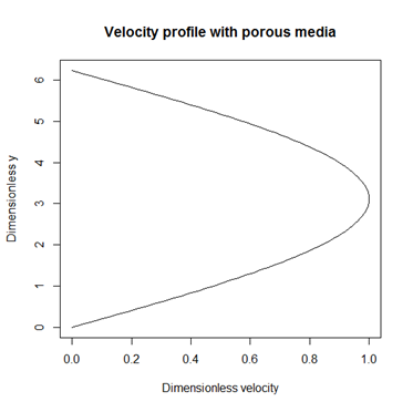
where the complex variable $z$  is $z\mathrm{<mo>=</mo>}{\omega }_1+z_0$ , where $z_0$  ranges from $0$  to $\pm 2Im\mathrm{<mo\; stretchy="false">(</mo>}{k}_1\mathrm{<mo\; stretchy="false">)</mo>}i$ . Since $k_1$  lies on $XA$ , ${\omega }_1$  is identical to $Re{k}_1$  and hence $z\mathrm{<mo>=</mo>}Re\mathrm{<mo\; stretchy="false">(</mo>}{k}_1\mathrm{<mo\; stretchy="false">)</mo>}+z_0$ . The following R code, with the library 'elliptic' was used to generate the velocity profile of Figure 3.⁶

Listing 2: Velocity profile of flow in porous medium

Figure 3 Velocity profile for flow in a porous channel bounded by flat plates.

The same code can be used if the equation $4s^3-g_{2}s-g_3\mathrm{<mo>=</mo>0}$  has a negative discriminant and $k_1$  is complex. In the event $k_1$  is real, the code should be modified so that the real axis is along the $y$  axis.

When we introduced the non-dimensional variables, we defined $y_{\star }\mathrm{<mo>=</mo>}y\mathrm{<mo>/</mo>}H$ . Therefore, $y_{\star }$  should range from 0 to 1. However, we notice in Figure 3 that it does not. We will introduce another transformation that brings the non-dimensional displacement variable between 0 and 1 after proving its validity.

Theorem 3: If we introduce a new non-dimensional displacement variable ${\tilde{y}}_{\star }$  defined as
${\tilde{y}}_{\star }\mathrm{<mo>=</mo>}\frac{y_{\star }}{\alpha }\mathrm{,}$
where $\alpha$ is a positive real number then this transformation keeps the form of equation (11) unchanged.

Proof: For sake of clarity, let us write the derivatives in full and re-introduce the $\prime \star \prime$  subscript for non-dimensional variables. Thus, equation (11) is written as
$\frac{d^2{u}_{\star }}{d{y}_{\star }{}^2}-A^2{u}_{\star }^2-B^2{u}_{\star }+C^2\mathrm{<mo>=</mo>0}$  (35)
If the non-dimensionalization of $y$  is done with $\alpha H$ , where $\alpha$  is a positive real number then
${\tilde{y}}_{\star }\mathrm{<mo>=</mo>}\frac{y}{\alpha H}\mathrm{<mo>=</mo>}\frac{y_{\star }}{\alpha }$
If $f$  is a function of $y$  then
$\frac{df}{d{y}_{\star }}\mathrm{<mo>=</mo>}\frac{df}{d{\tilde{y}}_{\star }}\frac{d{\tilde{y}}_{\star }}{d{y}_{\star }}\mathrm{<mo>=</mo>}\frac{1}{\alpha }\frac{df}{d{\tilde{y}}_{\star }}$
and hence
$\frac{d^2{u}_{\star }}{d{y}_{\star }{}^2}\mathrm{<mo>=</mo>}\frac{1}{{\alpha }^2}\frac{d^2{u}_{\star }}{d{\tilde{y}}_{\star }{}^2}$
If we denote the new dimensionless numbers with a tilde on top then from equations (8) to (10),
$\tilde{R}e\mathrm{<mo>=</mo>}\alpha Re$                                                                                       (36)
$\tilde{D}a\mathrm{<mo>=</mo>}\frac{Da}{{\alpha }^2}$                                                                                       (37)
$\tilde{J}\mathrm{<mo>=</mo>}J$                                                                                             (38)

The new pressure gradient is ${\tilde{G}}_{\star }\mathrm{<mo>=</mo>}\alpha G_{\star }$  while the new constants $\tilde{A}$ , $\tilde{B}$  and $\tilde{C}$  become
${\tilde{A}}^2\mathrm{<mo>=</mo>}\frac{F_0\epsilon \tilde{R}e}{\tilde{J}\sqrt{\tilde{D}a}}\mathrm{<mo>=</mo>}{\alpha }^2{A}^2$                                                                      (39)
${\tilde{B}}^2\mathrm{<mo>=</mo>}\frac{\epsilon }{\tilde{J}\tilde{D}a}\mathrm{<mo>=</mo>}{\alpha }^2{B}^2$                                                                         (40)
${\tilde{C}}^2\mathrm{<mo>=</mo>}\frac{{\epsilon }^2\tilde{R}e\tilde{G}}{\tilde{J}}\mathrm{<mo>=</mo>}{\alpha }^2{C}^2$                                                                     (41)

Therefore, equation (35) becomes,
$\frac{1}{{\alpha }^2}\frac{d^2{u}_{\star }}{d{\tilde{y}}_{\star }{}^2}-\frac{{\tilde{A}}^2}{{\alpha }^2}{u}_{\star }^2-\frac{{\tilde{B}}^2}{{\alpha }^2}{u}_{\star }+\frac{{\tilde{C}}^2}{{\alpha }^2}\mathrm{<mo>=</mo>0}$
or
$\frac{d^2{u}_{\star }}{d{\tilde{y}}_{\star }{}^2}-{\tilde{A}}^2{u}_{\star }^2-{\tilde{B}}^2{u}_{\star }+{\tilde{C}}^2\mathrm{<mo>=</mo>0}$
The vertical axis of the graph in Figure 3 extends from $0$  to $2Im\mathrm{<mo\; stretchy="false">(</mo>}{k}_1\mathrm{<mo\; stretchy="false">)</mo>}$ . To shrink it to $0$  to $1$ , we choose $\alpha \mathrm{<mo>=</mo>2<mo>*</mo>}Im\mathrm{<mo\; stretchy="false">(</mo>}{k}_1\mathrm{<mo\; stretchy="false">)</mo>}$ , in this case $6.232543$ . After changing the constants $A$ , $B$  and $C$  we proceed in similar fashion as before to get the plot in Figure 4.

Figure 4 Rescaled velocity profile for flow in a channel bounded by flat plates.

The code to generate the plot is

Listing 3: Velocity profile of flow in porous medium

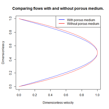
To compare the flow profiles with and without porous medium we choose the pressure gradient in the latter case so that the flow has the same peak velocity as in the former case. If we run the code in listing 4 after the one in listing 3, we can have the two profiles in the same plot as shown in Figure 5.

Listing 4: Comparison of velocity profiles

The flux of volume of fluid past a section of the channel is probably more important in practice than the velocity profile. In this section, I will calculate the flux in the channel. If $s$  denotes the transverse dimension of the channel then the flux $Q$  is $Q\mathrm{<mo>=</mo>}{\displaystyle {\int }_0^h}uds\mathrm{,}$

where $h$  is the width of the channel and $u$  is velocity of the fluid. If the channel does not have porous medium then
$u\mathrm{<mo>=</mo>}\frac{G}{2\mu }s\mathrm{<mo\; stretchy="false">(</mo>}h-s\mathrm{<mo\; stretchy="false">)</mo>}$
and hence the flux $Q_0$ is
$Q_0\mathrm{<mo>=</mo>}\frac{G{h}^3}{12\mu }$                                                                                       (42)
On the other hand if the channel is stuffed with porous medium then, the flux $Q_1$ is
$Q_1\mathrm{<mo>=</mo>}{\displaystyle {\int }_0^h}\frac{6}{A^2}\left[\wp \left(s+k_1\mathrm{<mo>|</mo>}\frac{1}{3}\left(A^2{C}^2+\frac{B^4}{4}\right)\mathrm{,}{g}_3\right)-\frac{B^2}{12}\right]ds$                    (43)
In terms of non-dimensional parameters $h\mathrm{<mo>=</mo>1}$  and hence $Q_0\mathrm{<mo>=</mo>}G\mathrm{<mo>/</mo><mo\; stretchy="false">(</mo>12}\mu \mathrm{<mo\; stretchy="false">)</mo>}$ . If we adjust pressure gradient so that peak velocity matches with that when porous medium is present, then code listing 5 gives $Q_0\mathrm{<mo>=</mo>0.6665793}$ . Carrying out the integration in equation (43) and noting that $s\mathrm{<mo>=</mo>}iy$ , we get $Q_1\mathrm{<mo>=</mo>0.6321661}$ . As expected from Figure 5, $Q_1\mathrm{<mo><</mo>}{Q}_0$ . Note that listing 5 is meant to be run after running listing (4).

Figure 5 Comparison of velocity profiles.

Listing 5: Calculation of flux,

There is another way to compute the flux of flow in a porous medium. It uses the relation between Weierstrass $\wp$  function and Weierstrass (not Riemann) $\zeta$ function.⁴
$\wp \mathrm{<mo\; stretchy="false">(</mo>}y\mathrm{<mo\; stretchy="false">)</mo><mo>=</mo>}-{\zeta }^{\text{'}}\mathrm{<mo\; stretchy="false">(</mo>}y\mathrm{<mo\; stretchy="false">)</mo>}$

Therefore, we get an analytical expression for $Q_1$ ,
$Q_1\mathrm{<mo>=</mo>}\frac{6}{A^2}\left[\zeta \mathrm{<mo\; stretchy="false">(</mo>}{k}_1\mathrm{<mo>|</mo>}{g}_2\mathrm{,}{g}_3\mathrm{<mo\; stretchy="false">)</mo>}-\zeta \mathrm{<mo\; stretchy="false">(</mo>1}+k_1\mathrm{<mo>|</mo>}{g}_2\mathrm{,}{g}_3\mathrm{<mo\; stretchy="false">)</mo>}\right]-\frac{B^2}{2A^2}$                          (45)

The library 'elliptic' allows us to evaluate Weierstrass $\zeta$  function. The listing 5, if run after listing 5 computes
$Q_1\mathrm{<mo>=</mo>0.6321664}$ .⁶

Listing 6: Another way to compute flux

None.

Author declares there is no conflict of interest in publishing the article.

1. DA Nield, SLM Junqueira, JL Lage. Forced convection in a fluid-saturated porous-medium with isothermal or isoflux boundaries. Journal of Fluid Mechanics. 1996;322:201−214.
2. Zaoli Guo, TS Zhao. Lattice Boltzmann model for incompressible flows through porous media. Phys Rev E Stat Nonlin Soft Matter Phys. 2002;66(3 pt 2B):036304.
3. ET Whittaker, GN Watson. A Course of Modern Analysis. UK: Cambridge University Press; 1927. p. 627.
4. Lawden Derek F. Elliptic functions and applications. Newyork: Springer-Verlag; 1989. p. 336.
5. M Abramowitz, IA Stegun. Handbook of Mathematical Functions with Formulas, Graphs, and Mathematical Tables. 10th printing, National Bureau of Standards, Applied Mathematical Series, USA. 1972. p. 470.
6. Hankin Robin KS. Introducing elliptic, an R package for elliptic and modular functions. Journal of Statistical Software. 2006;15(7):1−22.