Research Article Volume 2 Issue 1
Comparison of numerical and experimental results over a naca0025 airfoil undergoing separation
Amirhossein Ahadi,1,2
Pierre E Sullivan,2 M Ziad Saghir2
1Ryerson University, Canada
2Department of Mechanical and Industrial Engineering, University of Toronto, Canada
Correspondence: Amirhossein Ahadi, Graduate Level Instructor at Ryerson University, EPH-413, 87 Gerrard St East, Ryerson University, Toronto, Ontario, M5B2K3 Canada, Tel (647)7087764, Fax (647) 708-7764
Received: November 03, 2017 | Published: February 12, 2018
Citation: Ahadi A, Sullivan PE, Saghir MZ (2018) Comparison of Numerical and Experimental Results over a NACA0025 Airfoil Undergoing Separation. Fluid Mech Res Int 2(1): 00017. DOI: 10.15406/fmrij.2018.02.00017
Download PDF
Abstract
This paper examines unsteady numerical simulation of a three-dimensional flow over two different symmetric NACA airfoils. The airfoils are at various angles of attack and various low Reynolds numbers
. The Spalart-Allmaras, and
models, as well as LES and E-LES approaches are used and compared to experimental results. The capability of each turbulent model to capture characteristics at low Reynolds number is discussed. The main objective in this study is to capture the behavior of boundary-layer separation with respect to experiments at critical Reynolds numbers and then to establish a useful solution methodology describing transition in the boundary layer of airfoils accurately. Fully attached flow, boundary-layer separation, and boundary-layer with reattachment conditions are studied. Although LES and E-LES provide the highest computation cost, results show the accuracy of these methods at low Reynolds numbers (<150 x103). For higher Reynolds number, turbulence models provide a fair agreement with experiments; while the processing cost of LES method is very high. Finally, the impact of airfoil thickness, Reynolds number, and angle of attack on the boundary-layer separation and consequently airfoil performance are studied in detail.
Keywords: reynolds numbers, strouhal number, spalart-allmaras model, k-ε model, eppler 387 airfoil, NACA 0025 airfoil, smagorinsky
Abbreviations
Sep, separation; Max, maximum; LES, large eddy simulation; E-LES, embedded large eddy simulation; SAS, scale-adaptive simulation
Introduction
The performance of airfoils operating at low relative wind speeds (low Reynolds number) includes applications such as wind turbines, remotely piloted vehicles, sailplanes, human powered vehicles and high altitude devices.1‒3 At lower Reynolds numbers, both lift and drag characteristics are different from high Reynolds number flows.
Lin & Pauley2 studied unsteady boundary-layer separation from an Eppler 387 airfoil at low Reynolds number numerically and compared their results with wind tunnel measurements. They found unsteady large-scale structure might control the low-Reynolds-number separation bubble reattachment with small-scale turbulence playing a secondary role. Lin JCM,4 Drela{FormattingCitation},5 Drela & Giles6 used a fully coupled nonlinear system and predicted transitioning separation bubbles and their associated losses.
At low Reynolds numbers, flow separation occurs on the airfoils at small angles of attack, between
and
, with noticeable effects on airfoil efficiency. Moreover, with decreased Reynolds number, the length of the separation region decreased. When the maximum camber position was moved toward the trailing edge, the flow separation length was substantially reduced.7 Adding a burst control plate to increase the turbulent kinetic energy was found to reattach the shear layer to the airfoil surface.8
Measurements have shown that the boundary-layer separates downstream of an adverse pressure gradient, leading to the formation of a thin separation bubble and the second formed vortex loop retains its identity in the turbulent boundary layer and persists until the end of the test section.9 Experiments were performed for a range of low Reynolds numbers (50x103-200x103) and various angles of attack in a wind tunnel and over the NACA 0025 airfoil with a chord length c of 0.3m and a span of 0.88m. Boundary layer separation occurred over a large region on the upper surface of the airfoil for the entire range of angles of attack at Re=50x103 and Re=100x103.10,11 The results suggested that higher amplitude excitations might affect the airfoil performance at lower Reynolds numbers.12 In addition, it was pointed out that the magnitude of the acoustic excitation influence on the wake structure correlates with the extent of the improvement in the airfoil performance.
In this work, the boundary-layer behaviors of the symmetric airfoil NACA 0025 are studied numerically and are compared with experiments. The goal of this study is to find the most appropriate turbulence approaches for the simulation of boundary layer separation at different ranges of Reynolds number by comparing the Spalart-Allmaras and k-ε models and LES methods with experimental data.10
Governing Equations and Computational Models
Turbulent models
Spalart and allmaras model: The Spalart and Allmaras13 model is a modified turbulence model for aerospace applications involving wall-bounded flows. This has been found to have good performance for boundary layers subjected to adverse pressure gradients.14 In its original form, it is effectively a low-Reynolds number model, requiring the viscous-affected region of the boundary layer to be properly resolved and does not have non-local components in the equation, e.g. y+. The transported variable
is identical to the turbulent kinematic viscosity except in the viscous affected region,
(1)
Where
and
are, the production and destruction of turbulent viscosity respectively that occurs in the near-wall region. And,
and Cb2 are user-determined constants. The modified turbulent kinematic viscosity is set to zero at walls. When the mesh is generated appropriately to solve the laminar sub-layer, the wall shear stress is obtained from the laminar stress-strain equation.15
(2)
The
two-equation model: The two-equation models solve two separate transport equations and allow the turbulent velocity and length scales to be independently determined.16 The realizable
model was proposed by Shih et al.17 and was intended to solve some deficiencies of the traditional
models by adopting a new eddy-viscosity formula and a new dissipation equation, based on the dynamic equation of the mean-square vorticity fluctuation,
(3)
(4)
where,
are empirical constants for
model.
. Gk and Gb represent the generation of turbulent kinetic energy due to mean velocity gradients and buoyancy, respectively. YM is the contribution of the fluctuating dilatation in the compressible turbulence to the overall dissipation rate.18 In this model, the eddy viscosity is calculated from Eq. (6) with variable
.4,15
(5)
A0, As, and U* are functions of velocity gradients.
(6)
It is a semi-empirical model.16
To model transition from laminar to turbulent flow in this aerodynamic simulation, the approach of Eleni et al was used.16 The problem was simulated in Fluent after defining a laminar region (close to leading edge) and a turbulent zone. If the CD simulation result was greater than that of the experiment, the transition point moves closer to the trailing edge. This an iterative procedure until an accurate CD16,18 is obtained.
Large eddy simulation (LES) and embedded large eddy simulation (E-LES): LES still requires substantially finer meshes than those typically used for RANS calculations. In addition, LES has to be run for a sufficiently long flow-time to obtain stable statistics of the flow being modeled. As a result, the computational cost involved with LES is normally considerably higher than that for steady RANS calculations in terms of memory and CPU time.19,20
LES has had a limited impact on industrial CFD simulations, mainly because of its high computational costs. There are few technical applications where LES can be applied within the entire computational domain. Such flows are typically of low Reynolds numbers or with unimportant wall boundary layers. The high-resolution requirements for wall-bounded flows even at moderate Reynolds numbers have, in particular, severely limited the usage of LES.15,21
In order to allow the resolution of large turbulent structures in industrial flow simulations, hybrid models like Scale-Adaptive Simulation (SAS) have been employed. In such situations, zonal models are desirable, where a clear distinction between RANS and LES regions can be made, and where turbulence is converted from RANS to LES by suitable methods at the interface. One such approach is E-LES, where there are separate RANS and LES zones produced during the grid generation phase, then appropriate models for each zone are chosen and define the appropriate treatment at the interface. Usually, all RANS models can be used in the RANS region except for the Spalart-Allmaras one-equation model as it cannot provide the required turbulent length scale at the interface. Hence, for the RANS zone of the E-LES approach, realizable k-ε is used. In this model, the smaller scales and their interaction with the resolved scales have to be modeled through the sub grid scale term. The high-pass filtered Smagorinsky (HPF) eddy-viscosity model has been used here with has developed independently by Vreman (2003) and is closely related to the variational multiscale approach. It is known that by introducing a high-pass filtering the classical Smagorinsky closure could be applied without using any dynamic procedure in turbulent and transitional channel flow. In the HPF Smagorinsky, model the mean shear is removed by applying a high-pass filter to the grid-filtered velocity field. The turbulent eddy-viscosity and strain rate is then computed from the high-pass filtered velocity field rather than from the grid-filtered velocity field.
Numerical simulation
ANSYS Fluent was used in this study for numerical simulation. The Reynolds numbers for the simulations were Re=5, 10, 15, 20, 50, 100, 300 x 104 over a symmetric NACA airfoil 0025 at 0°, 5° and 10° is simulated here. The initial and boundary condition are defined based on standard room temperature and pressure.
Boundary conditions: The atmospheric far-field pressure with specified Mach number (calculated based on Reynolds number and the attack number) is used as boundary for all far field regions. The wall surface is taking no-sliding condition, and the initial condition of the flow field is setting in accordance with the free stream.8The geometry shown in Figure 1 is discretized using a 3D structured mesh of more than 350,000 quadrilateral Finite volumes for the RANS models while 4 million were used for the LES. The domain extends from 12 chords lengths upstream, upper and lower heights to 21 chord lengths downstream. To generate an elliptical 3D C-type grid, the wingspan is 12 chords.3,8,14,22‒24
The convergence criteria selected for this problem is 10-5 for the scaled absolute residuals of continuity, 10-6 for the scaled absolute residuals of momentum equations and lastly 10-9 for the energy equation. For cases simulated with RANS, the convergence criterion for turbulent viscosity was 10-5. Also, the convergence of airfoil’s lift and drag at the stationary result is considered.
Table 1 details the computational domain used including the number of cells in each direction, time step and quality of the mesh that has been used in this study. The boundary layer mesh has been also supplemented to divide the surface of the airfoil into two inner and outer regions. The inner region has a very fine mesh for E-LES over the entire domain. The governing equations are discretized over a domain based on element volumes. It should be note that the mesh and time sensitivity analysis have been performed for different cases and accordingly the time the total simulation and time step was different for various cases to ensure the mesh and time independency for each case. Accordingly, the solution imbalances at the starting point was less than 1%, and the residual levels 3E-6 is considered to converge in this study.
|
Case
|
Turbulent approach
|
Number of cells along the x,y and z directions
|
Cells attached to the airfoil surface
|
Quality of the mesh
|
Time step [s]
|
|
1
|
RANS models
|
80x80x30
|
918
|
Coarse
|
2 x10⁻¹
|
|
2
|
RANS models
|
100x100x36
|
3616
|
Fine
|
1 x10⁻²
|
|
3
|
LES
|
200x200x100
|
39876
|
Coarse
|
4 x10⁻⁴
|
|
4
|
LES
|
400x400x150
|
430870
|
Coarse
|
3 x10⁻⁶
|
|
5
|
E-LES
|
200x200x100
|
39876
|
Coarse
|
4 x10⁻⁴
|
|
7
|
E-LES
|
400x400x150
|
430870
|
Fine
|
3 x10⁻⁶
|
Table 1 The detail grid information of the numerical domain for various turbulent approaches
Numerical validation
For Re>150x103 the Spalart-Allmaras model predicts the flow separation fairly accurately. However, the E-LES approach is needed for lower Reynolds number. Consequently, the numerical results of the RANS model and E-LES approach were validated separately.
There are reliable experimental data10,25 for the NACA 0025 airfoil at Re=50, 100, 150 and 200 x103 at an angle of attack of 5°. The velocity profiles at different line around the airfoil has compared with the experimental results also and show 5 to 13% variation. The measured pressure distributions on the upper surface of the NACA 0025 airfoil are compared with the results here.
Figure 2 is the pressure distributions on the upper surface of the NACA 0025 airfoil when
at various Reynolds number with good agreement between the numerical and experimental results. While E-LES was used for all other Reynolds numbers, for Re=200 x103 the Spalart-Allmaras model is used and predicts the pressure distribution well. From Figure 2 there is the maximum deviation between the experimental and numerical results at the leading edge and the separation point.

Figure 2 Pressure distributions on the upper surface of the NACA 0025 airfoil when
at various Reynolds number.
Result and Discussion
Comparison of various turbulent approaches with experimental results at low and high Reynolds number
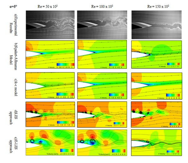
Figure 3A shows flow visualization of a single smoke wire located upstream of the airfoil at Re=50,100 and 150x103. In the case of non-reattached flow, large-scale structures are shed alternatively from the upper and lower sides of the airfoil wake. Whereas, for reattached flow the bubble forms on the upper surface, similar periodicity is observed in the wake.

Figure 3 Experimental result using smoke-wire flow visualization based on Yarusevych35 and Numerical results of wake and vortices at trailing edge and
, velocity along the x-direction [m/s].
The Spalart and Allmaras model Figure 3B shows only a small bubble at the trailing edge for Reynolds numbers less than 100 x103. It must be added that the Spalart and Allmaras model is in fair agreement for Re higher than 150x103; although no agreement with experiments was obtained at lower Re (>100 x103) based on Figure 3. The Spalart and Allmaras model and experimental pressure distributions on the upper surface of the NACA 0025 airfoil when
at Re=200 x103 show a similar behavior that proves the application of this turbulent model for Re=200x103. For
, Figure 3C, no separation can be detected. Despite this, the average pressure distribution around the airfoil for both turbulent models is similar for both methods.
LES shows better agreement with the experimental results (Figure 3D). Although the flow field predicted by LES at Re<150x103 was closer to experiments with respect to the formation of bubble; it does not provide a good agreement with experiments above 105. For example, bubble formation occurs only on the upper surface of the airfoil; whereas, according to the experiment at Re=100x103 strong separation occurs at both surfaces of the airfoil.
While LES can accurately capture transition in the boundary layer of a NACA0025 airfoil at low Reynolds number
and provide further insight into the physics of the separation bubble,26‒28 LES with a coarse mesh could not compute boundary layer separation precisely20 because there needs to be a very small time step
which is impossible with available resources. An alternative solution, which balances both cost and accuracy efficiency was E-LES. In this method, a very fine mesh may be used close to the airfoil boundary (inner region) where the flow is solved using LES; the outer region is calculated using a RANS model with a comparatively coarse mesh. As illustrated in Figure 3E, excellent agreement with experimental results are captured using E-LES for all experimental Reynolds numbers considered here. The Spalart-Allmaras turbulence model reasonably predicted the flow field at high Re numbers or high angle of attacks
(Figure 3) where the Spalart-Allmaras turbulence model predicted the formation of a bubble on the supper surface of the airfoil. On the other hand, the processing cost of the LES methods is prohibitively high for Re>100 x103
LES and E-LES showed accurate prediction of flow around the airfoils at low Re. On the other hand, the k-ε and Spalart-Allmaras models predict the time average pressure distribution in fair agreement with experimental results at high Reynolds numbers and angle of attacks. In addition, the Spalart-Allmaras model was able to capture the bubble formation at the trailing edge as did LES. At Re=3x10⁶, the boundary layer formed around the airfoil is fully turbulent3 and all turbulent models can reasonably predict the flow parameters. Consequently, LES approaches must be used for Re below critical Reynolds number (Recr=150x103) and for higher Re numbers, the Spalart-Allmaras model can predict the time average pressure distribution. E-LES was effective as it required about 1010 cells and a time step one to two orders of magnitude greater than LES’s time step thanks to the coarser mesh. It should be noted that the value of y+ for all of the cases where in the range of 0.7 to 1.45.
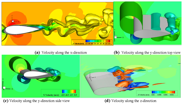
Three dimensional structure of the turbulent flow around NACA 0025 at Re=100x103 and
Figure 4 are the velocity contour and iso-surfaces velocity along the three axes for NACA 0025 at Re=100x103 and
. As observed in Figure 2, the strongest wake vortex shedding occurs at Re=100x 103, consequently, the 3D flow structure around the airfoil was analyzed. There is a clear 2-D velocity along the x and y directions. Iso-surface planes show no variation in the z-direction. Velocity fluctuations along the x-direction are evident under the trailing edge. Four bubbles can be seen in Figure 4B & 4C where the velocity along y-direction is plotted.

Figure 4 Velocity is o-surfaces along a) x-direction b) y-direction c) y-direction and d) z-directions for NACA 0025 at Re=100x103 and
.
Impact of reynolds number and angle of attack on boundary-layer separation
The reverse flow along the top surface of the airfoil was observed versus time at x/c=0.4 and Re=100x103(see Figure 3E and Re=100x103) with a roughly 5% overestimation of separation location compared with experimental results that indicated the separation at the maximum thickness location. Vortex structures are seen on the top surface of the airfoil when Re is less than Re=150x103. The flow reattached at Re=150 x103, in agreement with the experiments (see Figure 3 and Re=100x103).
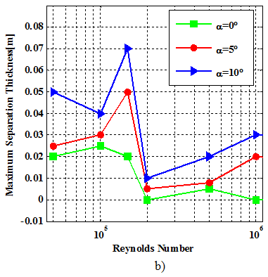
For Re numbers greater than 150x103, a separation bubble is formed on the upper surface close to the trailing edge. As the Reynolds number increases, the separation length decreases slightly, located between x/c=0.60 and 0.94. In contrast, decreasing the Reynolds number from 150x103 to 100x103 or 50x103, brings about significant changes in the boundary layer development Figure 5A. The maximum thickness of the separation zone at the upper side of the airfoil is responsible for boundary-layer separation for
. As shown in Figure 5B, maximum separation thickness occurs at 150x103. Also, for Re numbers greater than 20x103, a very thin (smaller than 3cm) separation zone is observed. Also, it can be seen that the most critical behavior occurs at Re around 100x103, before this Re number, maximum thickness increases and after that this parameter decreases. The critical flow behavior at the same Reynolds number was observed experimentally.29


Figure 5 a) Length and b) Thickness of the Separation as function of Reynolds number at various angles of attack, NACA0025.
To study flow separation around the airfoils at low Reynolds number and close to dynamic stall, LES and E-LES must be used. Figure 6 shows the NACA 0025 airfoil boundary-layer separation at Re=100 x103 for a range of angles of attack. Because of the thickness of this airfoil, separation is evident, even for zero angle of attack at x/c=0.48. However, the separated flow reattaches to the airfoil top surface at x/c=0.96. In contrast, reattachment at other angles of attack that causes the vortex shedding at the trailing edge cannot be detected. In addition, the thin but lengthy separated layer is the main reason for the constant-pressure region between x/c=0.78 and trailing edge.30 As angle of attack increases, the separation point moves towards the leading edge14 until reaching 15% of the chord for
. For higher Reynolds number at
, the separated boundary-layer reattaches to the airfoil surface, forming a laminar separation bubble.

Figure 6 Impact of different angle of attacks on the boundary-layer separation at Re=100x103
As seen in Figure 7A, the separation length over the NACA 0025 airfoil shows an approximate linear growth for increased angle of attack as well as for the maximum separation thickness (Figure 7B). In addition, it can be noted that a significant change in the flow field behaviour is detected comparing the first three lowest Re numbers and the three highest one in Figure 7A indicating two different regimes of the separation and the flow field.

Figure 7 a) Separation length, and b) Maximum separation thickness as a function of angle of attack for NACA0025 and different Reynolds numbers.
Velocity fluctuation of flow close to upper boundary
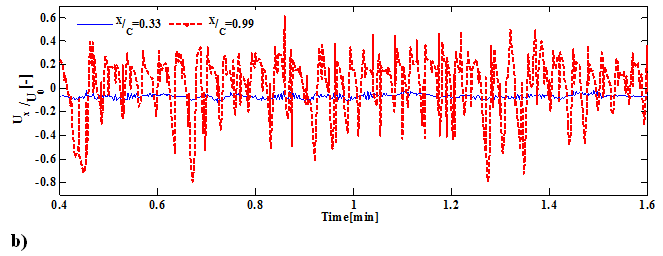
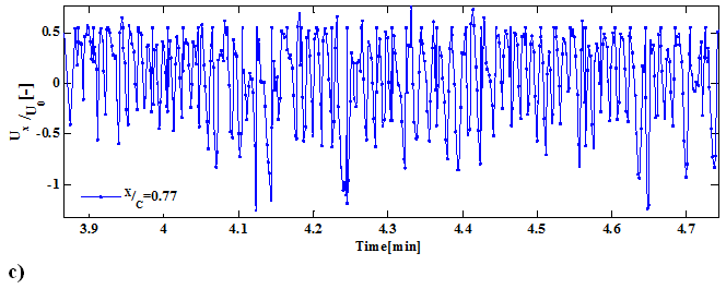
Figure 8 shows the streamwise velocity during transition for Re=50x103, 100x103, and 150x103 at different locations on top of the NACA 0025 airfoil. Initially, no significant fluctuations are observed in the laminar flow region until x/c=0.77 at Re=50x103. It can be claimed that as angle of attack increases, increment in the magnitude of the velocity fluctuation and decrement of its frequency occurs. At Re=50x103, the separated wake frequencies are roughly 27, 21 and 14 Hz for
respectively. For increased Reynolds number, the frequency of the streamwise velocity along x-direction increases. This observation can be seen in Figure 8B & 8C that these two diagrams represent the streamwise velocity at
. Beyond x/c=0.77 Figure 8C, the fluctuations were random. The highest frequency was observed at Figure 8C that represent the fluctuation of the velocity at x/c =0.77 when Re=150x 103(~110Hz).
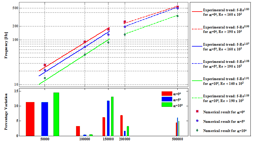
Yarusevych et al.10 have identified two distinct sets of data corresponding to the two flow regimes. They claimed that the fundamental frequency exhibits a power law dependency on the Reynolds number of the form
with respect to these two flow regimes. Particularly, the value of the exponent n (the power of Re in
) for Re<150 x103 varies from n obtained by curve fitting for Re>200x 103. They applied the power-law to the experimental data on airfoil profiles and the results are presented with solid lines in Figure 9 for both two regimes at various attack angels. As shown in the upper side of Figure 9, the values of the exponent n are collected from literature10,11,31,32 and used to find the best fits to numerical results. As it can be seen from the curve fits, the numerical data closely follow the power-law dependency established by experimental results.10,11,31,32 Nonetheless the second part of Figure 9 reports the percentage variations between the experimental and numerical results. The maximum and minimum variations are 14 and 1 percent for the flow at Re=50 x103 and
and the flow at Re=100 x103 and
respectively. In general, it can be seen that as Re increases the variation between the direct numerical simulation and the experimental data decreases. Finally, it can be claimed that the change of angle of attack does not have a pronounced impact on the behavior of the natural frequency.

Figure 9 Experimental11 and numerical variation of fundamental frequency f0 with Reynolds number at
.
The comparative analysis of the experimental results10,11,31,32 and the boundaries of the two flow regime proposed show a change of the flow regime leads to a change in the dependency of the fundamental frequency on the Reynolds number. It can be surveyed in more detail using the Strouhal number. Thus, the last parameter that is investigated in this study is a modified form of the Strouhal, the universal Strouhal number,
where d* represents the vertical distance between two vortices forming in the near-wake region and U0 is the mean velocity of the flow field. The variation of the resulting Strouhal number with the Reynolds number is shown in Figure 10 for both experimental10,11,31,32 and numerical results obtained in present study. It can be seen that both experimental and numerical results show minor scatter between St*=0.13 and 0.25; while, the average values for the numerical and experimental universal numerical Strouhal numbers are St*~0.1789 and 0.1718, which are in good agreement with each other and also the Strouhal number reported for cylinder, ~0.2.
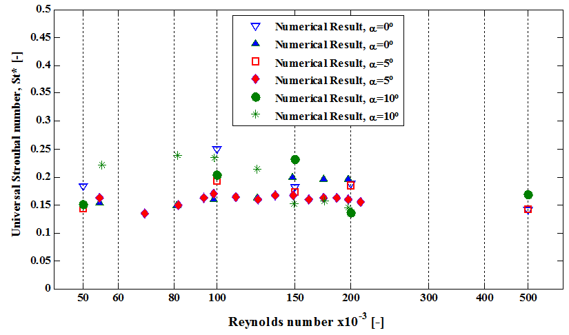
Figure 10 Universal vortex shedding frequency scaling based on wake flow geometry for experimental10,11,31,32 and numerical result obtained in this study.
Conclusion
Boundary layer and wake development on a NACA 0025 airfoil at low Reynolds numbers has been studied numerically. While different numerical approaches provide various results, LES and E-LES showed good agreement (especially E-LES). These methods only can be employed for low Re because of high computational cost for higher Re numbers. On the other side, the Spalart-Allmaras model captured the experimental data at higher Reynolds numbers or angles of attack in which LES approaches can be not used because of computational limits. The comparison between the numerical and experimental results suggests that for the LES approaches intensively fine mesh must be used to describe the boundary layer separation (even for low Reynolds numbers) while the RANS models cannot give accurate results.
The flow separation onset position and reattachment points on the airfoil contours have been calculated and compared on a NACA0025 airfoil at various angles of attack and Reynolds numbers. With LES and E-LES, separation at the zero angle of attack is captured. It can be seen that as Reynolds number increases, the airfoils demonstrate better aerodynamic performances based on this numerical analysis. Furthermore, it can be concluded that the aerodynamic performance of the airfoil increases as the separation point moves towards the trailing edge. Laminar boundary layer separation occurs on the upper surface of the NACA 0025 airfoil. While the flow reattaches to the airfoil surface at Re=150x103, for Re=100x103, the strongest wake shedding is observed in which separated shear layer fails to reattach to the airfoil surface.
Nomenclature:
|
CL
|
Normalized lift coefficient
|
|
CD
|
Normalized drag coefficient
|
|
c
|
Airfoil chord [m]
|
|
d
|
Distance to the closest wall [m]
|
|
f0
|
natural frequency [Hz]
|
|
Gk
|
Generation of turbulence kinetic energy due to the mean velocity gradients
|
|
Gb
|
Generation of turbulence kinetic energy due to buoyancy
|
|
gt
|
Min
|
|
I
|
Unit tensor
|
|
Mt
|
Turbulent Mach number
|
|
Mω,i
|
The molecular weight of species
|
|
Ls
|
The separation length [m]
|
|
p, p0
|
Local and free stream static pressure [Pa]
|
|
Re
|
Reynolds number
|
|
T
|
The static temperature [K]
|
|
Ts
|
The thickness of separation [m]
|
|
S
|
Magnitude of the vorticity [1/s]
|
|
Sm
|
Mass added to the continuous phase
|
|
U0
|
Free stream velocity in x-direction [m/s]
|
|
u,v
|
x and y fluctuating velocity components [m/s]
|
|
x,y
|
Stream wise and vertical coordinates
|
|
|
Angle of attack [deg]
|
|
|
Turbulent Prandtl numbers for k and
|
|
|
Viscosity [kg/ms]
|
|
|
Kinematic viscosity of air [m2/s]
|
|
|
Density of air [kg /m3]
|
|
|
Stress tensor [N/m2]
|
|
|
Wall vorticity at the trip [1/s]
|
|
|
Velocity difference between field point and at the trip [m/s]
|
|
|
Grid spacing along the wall at the trip [m]
|
|
Yi
|
The mass fraction of species
|
|
YM
|
Fluctuating dilatation contribution in compressible turbulence to the overall dissipation rate
|
Acknowledgement
This work was supported in part by the Natural Sciences and Engineering Research Council of Canada (NSERC). In addition, the authors acknowledge the support and guidance of Afshin Rahimi during this study.
Conflict of interest
Author declares that there is no conflict of interest.
References
- Selig M. Low Reynolds number airfoil design lecture notes. VKI Lecture Series, NATO Research and Technology Organization. Applied Vehicle Technology Panel, France; 2003. p. 1‒43.
- Lian Y, Shyy W. Laminar-turbulent transition of a low Reynolds number rigid or flexible airfoil. AIAA Journal. 2007;45(7):1501‒1513.
- Wang S, Ingham DB, Ma L, et al. Numerical investigations on dynamic stall of low Reynolds number flow around oscillating airfoils. Computers & Fluids. 2010;39(9):1529‒1541.
- Lin JCM, Pauley LL. Low-Reynolds-number separation on an airfoil. AIAA Journal. 1996;34(8):1570‒1577.
- Drela M. XFOIL: An Analysis and Design System for Low Reynolds Number Airfoils. Low Reynolds Number Aerodynamics. 1989. p. 1‒12.
- Drela M, Giles MB. Viscous-inviscid analysis of transonic and low Reynolds number airfoils. AIAA Journal. 2012;25(10):1347‒1355.
- Mateescu D, Abdo M. Analysis of flows past airfoils at very low Reynolds numbers. Proceedings of the Institution of Mechanical Engineers, Part G: Journal of Aerospace Engineering. 2010;224(7):757‒775.
- Grager T, Rothmayer A, Hu H. Stall Suppression of a Low-Reynolds-Number Airfoil with a Dynamic Burst Control Plate. 49th AIAA Aerospace Sciences Meeting including the New Horizons Forum and Aerospace Exposition. Florida, USA; 2011. p. 1‒10.
- Ma R, Liu P. Numerical Simulation of Low-Reynolds-Number and High-Lift Airfoil S1223. Proceedings of the World Congress on Engineering. UK; 2009. p. 1‒6.
- Yarusevych S, Sullivan PE, Kawall JG. On vortex shedding from an airfoil in low-Reynolds-number flows. Journal of Fluid Mechanics. 2009;632:245‒271.
- Yarusevych S, Sullivan PE, Kawall JG. Coherent structures in an airfoil boundary layer and wake at low Reynolds numbers. Physics of Fluids. 2006;18(4):44101‒44111.
- Yarusevych S, Sullivan PE, Kawall JG. Effect of acoustic excitation amplitude on airfoil boundary layer and wake development. AIAA Journal. 2007;45(4):760‒771.
- Spalart PR, Allmaras SR. A one equation turbulence model for aerodynamic flows. 30th Aerospace science meeting & exhibit. USA; 1992. p. 1‒23.
- Velazquez Araque L, Nozicka J. Numerical simulation of the fluid flow past an airfoil for an unmanned aerial vehicle. Thermodynamics and Fluid Mechanics. 2010;41:1‒16.
- ANSYS Fluent 14.0 User’s Guide. 2011. p. 2498.
- Eleni DC, Athanasios TI, Dionissios MP. Evaluation of the turbulence models for the simulation of the flow over a National Advisory Committee for Aeronautics (NACA) 0012 airfoil. Journal of Mechanical Engineering Research. 2012;4(3):100‒111.
- Shih TH, Liou WW, Shabbir A, et al. A new k-epsilon eddy viscosity model for high Reynolds number turbulent flows: Model development and validation. Computers and Fluids. 1995;24(3):227‒238.
- WU J. Evaluation of three turbulence models for the prediction of steady and unsteady airloads. AIAA, 27th Aerospace Sciences Meeting. Reno, USA; 1998. p. 1‒14.
- Lohász M, Rambaud P, Benocci C. LES simulation of ribbed square duct flow with Fluent and comparison with PIV data. Conference on Modeling Fluid Flow (CMFF’03), The 12th International Conference on Fluid Flow Technologies. Budapest, Hungary; 2003:1‒8.
- Xu T, Sullivan P, Paraschivoiu M. Fast Large-Eddy Simulation of Low Reynolds Number Flows over a NACA0025. Journal of Aircraft. 2010;47:328‒333.
- Le H, Moin P, Kim J. Direct numerical simulation of turbulent flow over a backward-facing step. Journal of Fluid Mechanics. 1997;330:349‒374.
- Tatineni M, Zhong X. Numerical Simulation of Unsteady Low-Reynolds-Number Separated Flows over Airfoils. APS Division of Fluid Dynamics Meeting Abstracts. 1996.
- Troshko AA, Hassan YA. A two-equation turbulence model of turbulent bubbly flows. International Journal of Multiphase Flow. 2001;27(11):1965‒2000.
- Jones DA, Clarke DB. Simulation of a Wing-Body Junction Experiment using the Fluent Code. DSTO Platforms Sciences Laboratory. Australia; 2005. p. 1‒55.
- Yarusevych S. Investigation of airfoil boundary layer and turbulent wake development at low Reynolds numbers. University of Toronto, Canada; 2006.
- Jaberi FA, Colucci PJ. Large eddy simulation of heat and mass transport in turbulent flows. Part 1: Velocity field. International Journal of Heat and Mass Transfer. 2003;46(10):1811‒1825.
- Shaw RH, Schumann U. Large-eddy simulation of turbulent flow above and within a forest. Boundary-Layer Meteorology. 1992;61(1‒2):47‒64.
- Yang Z, Voke PR. Large-eddy simulation of boundary-layer separation and transition at a change of surface curvature. Journal of Fluid Mechanics. 2001;439:305‒333.
- Yarusevych S, Kawall JG, Sullivan PE. Time-resolved surface pressure measurements within a separated flow region on an airfoil. Dynamics 37th AIAA Fluid Conference. USA: American Institute of Aeronautics and Astronautics; 2007. p. 2137‒2147.
- Yarusevych S, Kawall JG, Sullivan PE. Unsteady Separated Flow Characterization on Airfoils Using Time-Resolved Surface Pressure Measurements. AIAA Journal. 2008;46(2):508‒516.
- Roshko A. On the wake and drag of bluff bodies. Journal of the Aeronautical Sciences. 2002;22(2):124‒132.
- Roshko A. On the drag and shedding frequency of two-dimensional bluff bodies. USA: National Advisory Committee for Aeronautics; 1954. p. 31.

©2018 Ahadi, et al. This is an open access article distributed under the terms of the,
which
permits unrestricted use, distribution, and build upon your work non-commercially.


